Home Software Development Trash!
Sloppy Codes, Extra Sloppy
Between the Marlin paper coming out and a contract I’m currently working on, I started thinking about compression again a bit more recently. Friday night, I had an idea (it was quite a bad idea) about using a 16 entry Tunstall dictionary for binary alphabet entropy coding (with variable length output up to 8 bits in length) and using a byte shuffle to lookup the codes from a register in parallel when decoding, throwing in an adaption step.
My initial thought was that maybe it would be a good way to get a cheap compression win for encoding if the next input was a match or a literal in a fast LZ (and using a count trailing bits to count runs of multiple literals). I started to dismiss the idea as particularly useful by Saturday morning, thinking it was the product of too much Friday night cheese and craft beer after thinking about compression all week. However (quite quixotically), I decided to implement it anyway (standalone), because I had some neat ideas for the decoding implementation in particular that I wanted to try out. The implementation turned out quite interesting and I thought it would be neat to share the techniques involved. I also think it’s good to explore bad technical ideas sometimes in case you are surprised or discover something new, and to talk about the things that don’t work out.
As predicted, it ended up being fast (for an adaptive binary entropy coder), but quite terrible at getting much of a compression win. I call the results “Sloppy Coding” (sloppy codes, extra sloppy) and the repository is available here.
Firstly, I wrote a small Tunstall dictionary generator for binary alphabets that generated 16 entry dictionaries for 64 different probabilities and outputted tables for encoding/decoding as C/C++ code, so the tables can be shipped with the code and compiled inline. Each dictionary contains the binary output codes, the length of the codes, an extraction mask for each code and the probability of a bit being on or off in each node. This totals at 64 bytes (one cache line) for an entire dictionary (or 4K for all the dictionaries).
The encoded format itself packs 32 nibble words (dictionary references) into a 16 byte control word. First the low nibbles, then the high nibbles for the word are populated.
At decode time, we load the control word as well as the dictionary into a SSE registers, then split out the low nibbles:
__m128i dictionary     = _mm_loadu_si128( reinterpret_cast< const __m128i* >( decodingTable ) + dictionaryIndex * 4 );
__m128i extract        = _mm_loadu_si128( reinterpret_cast< const __m128i* >( decodingTable ) + dictionaryIndex * 4 + 1 );
__m128i counts         = _mm_loadu_si128( reinterpret_cast< const __m128i* >( decodingTable ) + dictionaryIndex * 4 + 2 );

__m128i  nibbles       = _mm_loadu_si128( reinterpret_cast< const __m128i* >( compressed ) );

__m128i  loNibbles     = _mm_and_si128( nibbles, nibbleMask );
Then we use PSHUFB to look up the dictionary values, bit lengths and extraction masks. We do a quick horizontal add with PSADBW to sum up the bit-lengths (we do the same for the high nibbles after):
__m128i  symbols   = _mm_shuffle_epi8( dictionary, loNibbles );
__m128i  mask      = _mm_shuffle_epi8( extract, loNibbles );
__m128i  count     = _mm_shuffle_epi8( counts, loNibbles );
__m128i  sumCounts = _mm_sad_epu8( count, zero );
Then there’s an extraction and output macro that extracts a 64 bit word from the symbols, masks, sums and counts, uses PEXT to get rid of the empty spaces between the values coming from the dictionary (this macro is used four times, twice each for the high and low nibbles). After that, it branchlessly outputs the compacted bits. We have at least 16 bits and at most 64 bits extracted at a time (and at most 7 bits left in the bit buffer). Note when repopulating the bit buffer at the end we have a small work around in case we end up with a shift right by 64 (that’s the first line of the last statement). The branch-less bit output, as well as the combination of PSHUFB and PEXT are some of the more interesting parts here (and a big part of what I wanted to try out). Similar code could be used to output Huffman codes for a small alphabet:
uint64_t symbolsExtract  =
	static_cast< uint64_t >( _mm_extract_epi64( symbols, extractIndex ) );
uint64_t maskExtract     =
	static_cast< uint64_t >( _mm_extract_epi64( mask, extractIndex ) );
uint64_t countExtract    =
	static_cast< uint64_t >( _mm_extract_epi64( sumCounts, extractIndex ) );

uint64_t compacted  = _pext_u64( symbolsExtract, maskExtract );

bitBuffer |= ( compacted << ( decompressedBits & 7 ) );

*reinterpret_cast< uint64_t* >( outBuffer + ( decompressedBits >> 3 ) ) = bitBuffer;

decompressedBits += countExtract;

bitBuffer = ( -( ( decompressedBits & 7 ) != 0 ) ) &
            ( compacted >> ( countExtract - ( decompressedBits & 7 ) ) );
After we’ve done all this for the high and low nibbles/high and low words, we adapt and choose a new dictionary. We do this by adding together all the probabilities (which are in the range 0 to 255), summing them together and dividing by 128 (no fancy rounding):
    __m128i probabilities = _mm_loadu_si128( reinterpret_cast< const __m128i* >( decodingTable ) + dictionaryIndex * 4 + 3 );
    __m128i loProbs       = _mm_shuffle_epi8( probabilities, loNibbles );
    __m128i sumLoProbs    = _mm_sad_epu8( loProbs, zero );
    __m128i hiProbs       = _mm_shuffle_epi8( probabilities, hiNibbles );
    __m128i sumHiProbs    = _mm_sad_epu8( hiProbs, zero );
    __m128i sumProbs      = _mm_add_epi32( sumHiProbs, sumLoProbs );

    dictionaryIndex = ( _mm_extract_epi32( sumProbs, 0 ) + _mm_extract_epi32( sumProbs, 2 ) ) >> 7;
Currently in the code there is no special handling at end of buffer (I just assume that there is extra space at the end of the buffer) because this is more of a (dis)proof of concept than anything else. The last up-to 7 bits in the bit buffer are flushed at the end.
The reason the decoder implementation is interesting to me is largely because of just how many of the operations can be done in parallel. We can look-up 16 dictionary codes at a time with PSHUFB and then pack the output of 8 of those looked up codes into a single 64bit word in two operations (an extract and a PEXT), which would usually take quite a lot of bit fiddling. The branchless output of that word to the output buffer is also nice, although it relies on some properties of the codes to work (mainly that there will always be more than 8 bits output, so we never have any of the previous bit buffer to worry about). Really, it feels like there is a lot of economy of motion here and the instructions fit together very neatly to do the job.
The one part that feels out of place to me though is having to work around there being a possible variable shift right by 64 bits when we store the residual in the bit buffer that wasn’t put in the output buffer. It would be nice if this wasn’t undefined behaviour (and processors implemented it the right way), but we can’t always get what we want.
Results
For testing, I generated 128 megabytes of randomly set bits (multiple times, according to various probability distributions), as well as a one that used a sine wave to vary the probability distribution (to make sure that it was adapting). Compression and decompression speed are in megabytes (the old fashioned 10242 variety) averaged over 15 runs. Bench-marking machine is my usual Haswell i7 4790.
The compression ratio for the outlying probabilities (0 to 1) achieves at or very close to the theoretical optimum capable of the coder (which is fairly far from entropy) and the middle most probabilities are not too far away from achieving entropy (even if they slightly gain information). But the ratios just outside the middle don’t drop quite fast enough for any savings in most scenarios and stay stubbornly high. A much larger dictionary, with longer maximum output codes, would offer considerably more savings at the cost of losing our neat implementation tricks and performant adaption (but Tunstall coding is already a fairly known quantity). There’s also the matter of how imprecise our probability model is and compared to most other adaptive coders, we don’t adapt per symbol.
Speedwise, (remembering that our actual output symbols are bits), for decompression we’re far faster than an adaptive binary arithmetic coder is capable of, given we’re outputting multiple bits per cycle (where as a binary arithmetic coder is going to take multiple cycles for a single bit). But that’s not saying much, given how relatively far we are away from entropy (where a binary arithmetic closer gets as close as its precision will allow).
| Probability | Compression Speed | Encoded Size | Ratio | Decompression Speed |
|---|---|---|---|---|
| 0 | 206.230639 | 67114272 | 0.50004 | 2158.874927 |
| 0.066667 | 175.3852 | 79162256 | 0.589805 | 1831.462974 |
| 0.133333 | 151.631986 | 91572032 | 0.682265 | 1586.54503 |
| 0.2 | 132.081896 | 104868416 | 0.781331 | 1377.348473 |
| 0.266667 | 117.898678 | 117748768 | 0.877297 | 1236.169277 |
| 0.333333 | 108.803616 | 127463824 | 0.949679 | 1141.881051 |
| 0.4 | 104.331363 | 133059200 | 0.991368 | 1084.070366 |
| 0.466667 | 102.554293 | 134885904 | 1.004978 | 1057.176446 |
| 0.533333 | 102.718932 | 134931136 | 1.005315 | 1066.073632 |
| 0.6 | 104.353041 | 133057584 | 0.991356 | 1092.383074 |
| 0.666667 | 108.918791 | 127351120 | 0.94884 | 1143.198439 |
| 0.733333 | 118.245568 | 117570320 | 0.875967 | 1226.966374 |
| 0.8 | 132.864274 | 104712784 | 0.780171 | 1389.678224 |
| 0.866667 | 151.684972 | 91559024 | 0.682168 | 1585.006786 |
| 0.933333 | 174.659716 | 79162864 | 0.589809 | 1830.458242 |
| 1 | 205.484085 | 67108880 | 0.5 | 2162.718762 |
| Sine Wave | 140.850482 | 98377072 | 0.732966 | 1461.307419 |
Tags: Compression Sloppy SSE
Boondoggle, the VR Music Visualizer
When I got my Oculus in June, one of the things that struck me was that the experiences that I enjoyed most were those where you could relax and just enjoy being somewhere else. It reminded me a lot of one of my favourite ways of relaxing; putting on headphones and losing myself in some music. I’d also been looking at shadertoy and many cool demos coming through on my twitter feed and wanted to have a bit of a try of some of the neat ray marching techniques.
So the basic idea that followed from this was to create a music visualization framework that could capture audio currently playing on the desktop (as to work with any music player that wasn’t running a DRM stream), do a bit of signal processing on it and then output pretty ray marched visuals on the HMD.
Here’s a capture of a visualizer effect running in a Window:
And here’s one in the HMD rendering view:
This post basically goes through how I went about that, as well as the ins and outs of one visualizer effect I’m pretty happy with. I should be clear though, this is a work in progress and a spare time project that has often been left for weeks at a time (and it’s in a definite state of flux). The current source is on github and will be updated sporadically as I experiment. There is also a binary release. There is a lot to be covered here, so in some sections I will be glossing over things (feel free to email me, leave a comment or contact me on twitter if there is any detail you would like clarified).
Basic Architecture
The visualizer framework has two main components; the visualizer run-time itself, and a compiler that takes a JSON file that references a bundle a bunch of HLSL shaders and textures and turns them into visualizer effects package used by the run-time. The compiler turn around time is pretty quick, so you can see effects changes quite quickly (iteration time isn’t quite shadertoy good, but still pretty reasonable). The targeted platforms are Windows, D3D 11, and the Oculus SDK (if you don’t have the Oculus runtime installed or a HMD connected, it will render into a window, but the target is definitely a HMD; the future plan is to add OpenVR SDK support too).
I used Branimir Karadzic’s GENie to generate Visual Studio projects (currently the only target I support), because it was a bit easier than building and maintaining the projects by hand. Apart from the Oculus SDK and platform dependencies, all external code has been copied into the repository and is compiled directly as part of the build. Microsoft’s DDS loader from DirectXTex is used to load textures, KISS FFT is used for signal processing and JSON is parsed with Neil Henning’s json.h.
Originally I was going to capture and process the audio on a separate thread, but given how light the CPU requirements for the audio capturing/processing are and that we aren’t spending much CPU time on anything else, everything ended up done on a single thread, with the audio being polled every frame.
Handling the Audio
Capturing audio from the desktop on Windows is interesting. The capture itself is done using WASAPI with a loop-back capture client running on the default device. This pretty much allows us to capture whatever is rendering on a device that isn’t exclusive or DRM’d (and we make sure the data is coerced to floating point if it isn’t already).
One of the caveats to this is that capture doesn’t work when nothing is playing on the device, so we also create a non-exclusive render device and play silence on it at the same time.
Every frame we poll to A) play silence on the device if there is room in the playback buffer and B) capture any sound data packets currently to be played to the device by copying them into a circular buffer per channel (we do this as we only copy out the first two channels of the audio in case the device is actually surround sound, mono is handled by duplication). This works very well as long as you maintain a high enough frame-rate to capture every packet coming out of the device; the case where a packet is missed is handled by starting from scratch in the circular buffer.
Audio processing is tied to the first power-of-two number of samples that allow us to capture our minimum frequency for processing (50hz). The circular buffer is twice this size and instead of using the head of the buffer to do the audio processing every frame, we use either the low or high halves of the circular buffer whenever they are full.
When we capture one of those roughly-50hz shaped blocks, we do a number of processing steps to get the data ready to pass off to the shaders:
- Calculate the RMS on all the samples in the block per channel to get an estimate of how loud that channel is. Also a logarithmic version of this cut off at a noise floor to get a more human friendly measure. These values are smoothed using an exponential moving average to make them more visually appealing in the shaders.
- Run a Windowing function (Hanning, but this can be changed to any other Generalized Hamming Window relatively easily) prior to the FFT to take out any spurious frequency data that would come from using a finite/non-wrapping FFT window. Note, we don’t do overlapping FFT windows as this works fine for visualization purposes.
- Run a real FFT per channel using KISS FFT.
- Divide the frequency bins into 16 buckets based on a modified version of the formula here and work out the maximum magnitude of any frequency bin in the bucket, convert it to a log scale, cut off at the noise floor and smooth it using an exponential moving average with previous values. This works a lot better in the shader than putting the whole FFT into a texture and dealing with it.
- Copy the audio channel data and the amplitude of each frequency bin in the FFT into a small texture. Note, this uses a fairly slow path for copying, but the texture is tiny so it has very little impact.
Oculus Integration
I was very impressed with the Oculus SDK and just how simple it was to integrate. The SDK allows you to create texture swap chains that you can render to in D3D and then pass off to a compositor for display (as well as getting back a mirror texture to display in a Window) and this is very simple and integrates well.
In terms of geometry, you get the tan of all the half angles for an off-axis frustum per eye, as well as the poses per eye as a quaternion orientation and position. Because we’re ray-marching, we aren’t going to use a traditional projection matrix, but instead some values that will make it easy to create a ray direction from screen coordinates:
// Create rotation adjusted for handedness etc
XMVECTOR rotation = XMVectorSet( -eyePose.Orientation.x,
                                 -eyePose.Orientation.y,
                                 eyePose.Orientation.z,
                                 eyePose.Orientation.w );

// Upper left corner of the view frustum at z of 1. Note, z positive, left handed.
XMVECTOR rayScreenUpperLeft = XMVector3Rotate( XMVectorSet( -fov.LeftTan,
                                                            fov.UpTan,
                                                            1.0f,
                                                            0.0f ),

// Right direction scaled to width of the frustum at z of 1.
XMVECTOR rayScreenRight = XMVector3Rotate( XMVectorSet( fov.LeftTan + fov.RightTan,
                                                        0.0f,
                                                        0.0f,
                                                        0.0f ),
                                           rotation );

// Down direction scaled to height of the frustum at z of 1.
XMVECTOR rayScreenDown = XMVector3Rotate( XMVectorSet( 0.0f,
                                                       -( fov.DownTan + fov.UpTan ),
                                                       0.0f,
                                                       0.0f ),
                                          rotation );
In the shader, we’ll use the eye position we get from the Oculus SDK as the ray origin and use these values to create a ray direction. Oculus use meters as their unit, so I decided to stick with that.
Oculus also takes care of the GPU sync, time warp (if needed, when you begin your frame and get the HMD position, you also get a time value that you then feed in when you submit the frame), distortion and chromatic aberration correction.
File Format
At the content build step, I package everything into a single file that gets memory mapped at run-time. I use the same relative addressing trick used by Per Vognsen’s GOB, with a bit of C++ syntax sugar. The actual structures in the file are traversed in-place both at load time (to load the required resources into D3D) and per frame.
Rendering
Per frame, we basically get an effect id. Given that effect id, we look-up the corresponding shader and set any corresponding textures/samplers (including potentially the sound texture); all of this information comes directly out of the memory mapped file and indexes corresponding arrays of shaders/textures.
While I support off-screen procedural textures that can be generated either at load time or every frame, I haven’t actually used this feature yet, so it’s a not tested. Currently these use a specified size, but at some stage I plan to make these correspond to the HMD resolution.
Each package has a single vertex quad shader that is expected to generate a full-screen triangle without any input vertex or index data (it creates the coordinates directly from the ids). We never load any mesh data at all into index or vertex buffers for rendering, as all geometry will be ray-marched directly in the pixel shader.
Another thing on the to-do list is to support variable resolution rendering to avoid missed frames and allow super-sampling on higher-end hardware. I currently have the minimum required card for the Rift (a R9 290), so the effects I have so far are targeted to hit 90hz with some small margin of safety at the Rift’s default render resolution on that hardware (I’ve also tested outside VR on a nvidia GTX 970M).
The Visualizer Effect in the Video
The visualizer effect in the video is derived from my first test-bed effect (in the source code), but was my first attempt at focusing on creating something aesthetically pleasing as opposed to just playing around (my name for the effect is “glowing blobby bars”, by the way). It’s based on the very simple frequency-bars visualization you see in pretty much every music player.
To get a grounding for this, I recommend reading Inigo Quilez article on ray marching with distance functions and looking at Mercury’s SDF library.
Each bar’s height comes from one of the 16 frequency buckets we created in the audio step, with the bars to either side coming from the respective stereo channel.
To ray march this, we create a signed distance function based on a rounded box and we use a modulus operation to repeat it, which creates a grid (where we expect that if a point is within a grid box, it is closest to the contents of the grid box than other those in other grid boxes) . We can also get the current grid coordinates by doing an integer division, which is what we do to select the frequency bucket to get the bar’s height and material (and also use as the material id).
There is a slight caveat to this in that sometimes the height difference between two bars is such that a bar in another grid slot may actually be closer than the bar in the current grid slot. To avoid this, we simply space the bars conservatively relative to their maximum possible height difference. The height is actually tied to the cubed log-amplitude of the frequency bucket to make the movement a bit more dramatic.
To create the blobby effect, we actually do two things. Firstly, we twist the bars using a 2D rotation based on the current y coordinate, which adds a bit more visually interesting detail, especially on tall bars. We also use a displacement function based on overlapping sine waves of different frequencies and phases tied to the current position and time, with an amplitude tied to the different frequency bins. Here’s the code for the displacement below:
float scale = 0.25f / NoiseFloorDbSPL;

// Choose the left stereo channel
if ( from.x < 0 )
{
    lowFrequency = 1 - ( SoundFrequencyBuckets[ 0 ].x +
                         SoundFrequencyBuckets[ 1 ].x +
                         SoundFrequencyBuckets[ 2 ].x +
                         SoundFrequencyBuckets[ 3 ].x ) * scale;
    midLowFrequency = 1 - ( SoundFrequencyBuckets[ 4 ].x +
                            SoundFrequencyBuckets[ 5 ].x +
                            SoundFrequencyBuckets[ 6 ].x +
                            SoundFrequencyBuckets[ 7 ].x ) * scale;
    midHighFrequency = 1 - ( SoundFrequencyBuckets[ 8 ].x +
                             SoundFrequencyBuckets[ 9 ].x +
                             SoundFrequencyBuckets[ 10 ].x +
                             SoundFrequencyBuckets[ 11 ].x ) * scale;
    highFrequency = 1 - ( SoundFrequencyBuckets[ 12 ].x +
                          SoundFrequencyBuckets[ 13 ].y +
                          SoundFrequencyBuckets[ 14 ].x +
                          SoundFrequencyBuckets[ 15 ].x ) * scale;
}
else // right stereo channel
{
    lowFrequency = 1 - ( SoundFrequencyBuckets[ 0 ].y +
                         SoundFrequencyBuckets[ 1 ].y +
                         SoundFrequencyBuckets[ 2 ].y +
                         SoundFrequencyBuckets[ 3 ].y ) * scale;
    midLowFrequency = 1 - ( SoundFrequencyBuckets[ 4 ].y +
                            SoundFrequencyBuckets[ 5 ].y +
                            SoundFrequencyBuckets[ 6 ].y +
                            SoundFrequencyBuckets[ 7 ].y ) * scale;
    midHighFrequency = 1 - ( SoundFrequencyBuckets[ 8 ].y +
                             SoundFrequencyBuckets[ 9 ].y +
                             SoundFrequencyBuckets[ 10 ].y +
                             SoundFrequencyBuckets[ 11 ].y ) * scale;
    highFrequency = 1 - ( SoundFrequencyBuckets[ 12 ].y +
                          SoundFrequencyBuckets[ 13 ].y +
                          SoundFrequencyBuckets[ 14 ].y +
                          SoundFrequencyBuckets[ 15 ].y ) * scale;
}

float distortion = lowFrequency * lowFrequency * 0.8 *
                        sin( 1.24 * from.x + Time ) *
                        sin( 1.25 * from.y + Time * 0.9f ) *
                        sin( 1.26 * from.z + Time * 1.1f ) +
                   midLowFrequency * midLowFrequency * midLowFrequency * 0.4 *
                       sin( 3.0 * from.x + Time * 1.5 ) *
                       sin( 3.1 * from.y + Time * 1.3f ) *
                       sin( 3.2 * from.z + -Time * 1.6f ) +
                   pow( midHighFrequency, 4.0 ) * 0.5 *
                       sin( 5.71 * from.x + Time * 2.5 ) *
                       sin( 5.72 * from.y + -Time * 2.3f ) *
                       sin( 5.73 * from.z + Time * 2.6f ) +
                   pow( highFrequency, 5.0 ) * 0.7 *
                       sin( 9.21 * from.x + -Time * 4.5 ) *
                       sin( 9.22 * from.y + Time * 4.3f ) *
                       sin( 9.23 * from.z + Time * 4.6f ) *
                   ( from.x < 0 ? -1 : 1 );
There are a few issues with this displacement; first it’s not a proper distance bound so sphere tracing can sometimes fail here. Edward Kmett pointed out to me that you can make it work by reducing the distance you move along the ray relative to the maximum derivative of the displacement function, but in practice that ends up too expensive in this case, so we live with the odd artifact where sometimes a ray will teleport through a thin blob.
Due to this problem with the distance bound, we can’t use the relaxed sphere tracing in the enhanced sphere tracing paper, but we do make our minimum distance cut-off relative to the radius of the pixel along the ray. Because the distance function is light enough here, we don’t actually limit the maximum number of iterations we use in the sphere tracing (the pixel radius cut-off actually puts a reasonable bound on this anyway with our relatively short view distance of 150 meters).
Also, the displacement function is relatively heavy, but luckily we’re only computing it (and the entire distance function) for only the bar within the current grid area.
Another issue is that with enough distance from the origin, or a large enough time, things will start to break down numerically. In practice, this hasn’t been a problem, even with the effect running for over an hour. We also reset the time every time the effect changes (currently changing is manual, but I plan to add a timer and transitions).
Lighting is from a directional light which shifts slowly with time. There is a fairly standard GGX BRDF that I use for shading, but in this scene the actual colour of the bars is mostly ambient (to try and give the impression that the bars are emissive/glowing). The material colours/physically based rendering attributes come from constant arrays indexed by the material index of the closest object returned by the distance function.
For the fog, the first trick we use is from Inigo’s better fog, where we factor the light into the fog (I don’t use the height in the fog here). The colour of the fog is tied to the sound RMS loudness we calculated earlier, as well as a time factor:
float3 soundColor = float3( 0.43 + 0.3 * cos( Time * 0.1 ),
                            0.45 + 0.3 * sin( 2.0 * M_PI * SoundRMS.x ),
                            0.47 + 0.3 * cos( 2.0 * M_PI * SoundRMS.y ) );
This gives us a nice movement through a variety of colour ranges as the loudness of the music changes. Because of the exponential moving average smoothing we apply during the audio processing, the changes aren’t too aggressive (but be aware, this is is still relatively rapid flashing light).
The glow on the bars isn’t a post process and is calculated from the distance function while ray marching. To do this, we take the size of the movement along the previous ray and the ambient colour of the closest bar and sum like this every ray step:
glow += previousDistance * Ambient[ ( uint )distance.y ] / ( 1 + distance.x * distance.x );
At the end we divide by the maximum ray distance and multiply by a constant factor to put the glow into a reasonable range. Then we add it on top of the final colour at the end. The glow gives the impression of the bars being emissive, but also enhances the fog effect quite a bit.
One optimisation we do to the ray marching is to terminate rays early if they go beyond the maximum or minimum height of the bars (plus some slop distance for displacement). Past this range the glow contribution also tends to be quite small, so it hasn’t been a problem with the marching calculations for the glow.
Shameless Plug
If you like anything here and need some work done, I’m available for freelance work via my business Burning Candle Software!
Tags:
Starting Something New
Building software is something that I love, it’s been my hobby for over 20 years and my profession for only a few years less. I do have a life (with a family and hobbies that brings me joy) outside of it, but it is one of my true pleasures.
It offers a lot: it’s a craft you can hone and perfect; there are aspects of science, maths, creativity, logic and humanity all balanced together; it can give you an enormous sense of achievement; it gives you the chance to communicate and collaborate with amazing people and it allows you a lot of mental space to go roaming.
But I’ve been feeling restless for a long time, because I haven’t felt like I’ve been participating with my peers enough. The things I’ve worked on professionally, in the last few years, have been largely been things that lived behind closed doors. The circle of people I interacted with professionally was quite small.
Another ennui factor is that I haven’t felt the space to be able to pursue my own ideas. I don’t believe that any one idea, by itself, is that valuable. But being able to explore it and turn it into something real is.
My little side projects over the last few years have started to scratch that itch. But they, LZSSE in particular, were also enough to make me understand that I needed more.
Because of that, I’ve decided to start my own business, Burning Candle Software. Part of what we’ll be doing will give me the chance to work with more of you (contracting, development services, consulting, mentoring). I’ve worked remotely before (both internationally and interstate), so that isn’t an obstacle for me. If you have a problem that needs solving and you think I’d be a good fit, reach out. Even if we can’t come to an arrangement, I’m always happy to help where I can.
Some of that might include expanding or integrating the technology (or similar things) from this blog. If you’re interested in that, I’d be very happy to hear from you.
It will also give me the freedom to choose when to pursue my own ideas, some of which will end up as open source and contributed back to the community (with the usual technical detail blog posts) and maybe even one or two will become commercial (or maybe both at the same time).
Finally, I’m looking forward to getting more in touch with the local development community in Perth, who I have not had much of a chance to engage with in recent years. It will be fun both learning from them and providing mentoring where I can.
I’ve had a pretty varied career; I’ve worked in games, I’ve done focused graphics and computational geometry research in a corporate lab environment, I’ve lead teams, I’ve been involved with engineering large scale projects (like smart card systems), built bespoke and packaged software used all over the world and been the lead developer/quantitative analyst for an algorithmic trading firm. I’ve had experience in areas like graphics, performance optimization, distributed systems, high performance networking, compression, image processing, machine learning, natural language processing, geographic systems and am hoping to get experience in many more (VR!).
This is new for me and that’s a little intimidating. But I’m here and I want to contribute.
A Simple Guide to Moving Data into R
As developers, it’s important to understand what is going on in the software we implement, whether we are designing a new algorithm, or looking at how an existing implementation is interacting with a particular data set (or even gain insights into the data set itself). R is something that I use a fair bit these days for generating easy visualizations, especially when I’m looking at say, how to build a compression algorithm. I’ve been using it for around 3 years now, with good results. It’s also good for more advanced analysis, data processing and building content for presentations or the web.
R has quite strong builtin capabilities, as well as a massive library of plugin packages. You can do visualizations from simple plots to interactive 3D (that can be exported to render on a web page in Web GL, via the rgl package). There are also functions for massaging data, full blown statistical analysis and machine learning. Microsoft has just released a free Visual Studio integration and is strongly pushing R support into it’s product range, but R has a strong open ecosystem, is available on every common desktop OS and it is usable via a number of GUI tools, IDEs and the command line.
I’m not going to teach you how to use the language as much as show the way I use it in combination with software I’m actually developing. The language is pretty easy to pick up (and you don’t really need to learn that much, there are ready-to-copy of cookbooks that will get you most of the way there).
How I Use R
The typical way I use R is short scripts that take an output file, generate a visualization to a file, then open that file for viewing (R has built in display capabilities, but there are some limitations when running scripts outside of the GUI/IDE environments). It is possible to automate running the script (there is a command line utility called RScript that you can launch from your own code and it also allows command line parameters to be passed to the script) and it’s even possible to write scripts that take piped data (either from stdin or opening a local pipe).
One of the biggest reasons I use R is because getting data in (and out) is very simple. In fact, if you come from a C/C++ background, where even the simplest data parsing is a detail ridden chore, the simplicity with which R lets you import data to work with straight away can be empowering. R also has built in help, so if you get stuck, you can look at the help for any function in the REPL simply by prefixing it with a question mark.
The way I usually get data into R is loading a delimited file (comma, tab and custom delimited are all supported) into a data frame object. Data frames are essentially tables, they have rows and columns, where each row and column has a name (although, typically the names for the rows are ascending integers). One of the great things about doing things this way is that R will handle all the data typing automatically, columns with real numbers will work as such, as will strings (provided you get your delimiting right!). You can then access rows and columns either by name or by index ordinal (there is also slicing), or individual cells.
Quite often I’ll temporarily add a statically allocated array to code to generate a histogram following what a particular algorithm is doing in code, then flush/dump it out to a file when I’ve collected the data. At other times it’s possible to just append to the file every time you want to put out a data point, as a kind of event logging (you generally only need to write a single line).
Example
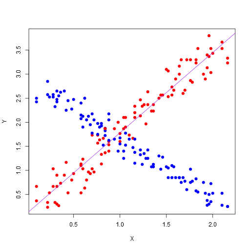
Here’s a very simple example. Firstly, here is a C program that generates 2 points using two jittered linear functions (we re-use the X component, but we’re generating two separate Ys) and outputs them as simple tab separated data with column headings in the first row. Each linear function has a matching color (red or blue).
#include <stdlib.h>
#include <stdio.h>

int main()
{
    printf( "X\tY\tColor\n" );

    for ( int where = 0; where < 100; ++where )
    {
        double x = ( where + ( rand() % 15 ) ) / 50.0;
        double y1 = ( where + ( rand() % 20 ) ) / 30.0;
        double y2 = ( ( 100 - where ) + ( rand() % 20 ) ) / 40.0;

        printf( "%G\t%G\tred\n", x, y1 );
        printf( "%G\t%G\tblue\n", x, y2 );
    }

    return 0;
}
We then pipe the standard output of this into a file (let’s call it “data.txt”). What does the R Script look like to turn this data into a scatter plot?
dataTable <- read.table("data.txt", header=TRUE)

png("data.png", width = 512, height = 512, type = c("cairo"), antialias=c("gray"))

plot(x = dataTable$X,
     y = dataTable$Y,
     pch = 19,
     xlab = "X",
     ylab = "Y",
     col = as.character(dataTable$Color))

justRed <- subset(dataTable, Color == "red")

abline(lm(formula=justRed$Y ~ justRed$X), col="purple")

dev.off()

browseURL("data.png", browser=NULL)
Here’s what we’re doing:
-
Use the read.table function to read the data.txt into a data frame. We’re using the first row of the data as column headers to name the columns in the data frame. Note, there are also CSV and Excel loads you can do here, or you can use a custom separator. The read.table uses any white space as a separator by default.
-
Create a device that will render to a PNG file, with a width of 512, height of 512, using Cairo for rendering and a quite simple antialiasing (this makes for prettier graphs than using native rendering). Note, you can display these directly in the R GUI; the Visual Studio integration actually shows the graph in a pane inside Visual Studio.
-
Draw a scatter plot. We’ve used the “X” and “Y” columns from our loaded data frame, as well as the colors we provided for the individual points. We’ve also set the shape of the plot points (with pch=19). Note, you can also access columns by position and use the column names as graph labels.
-
After that, we’ve selected the subset of our data where the Color column is “red” into the data frame and drawn a line using a linear regression model (with the simple formula of the Y mapping to X).
-
Switch off the device, which will flush the file out.
-
Open up the file with the associated viewer (this might only work on Windows and is an optional step).
Here’s the resulting image:
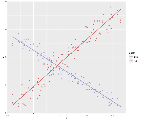
Note, this is the most basic plotting. There are many plotting libraries that produce better images, for example, here is ggplot2 using the following code (note, you’ll need to make sure you have ggplot2 package installed before you can do this):
library(ggplot2)

dataTable <- read.table("data.txt", header=TRUE)

png("data.png", width = 600, height = 512, type = c("cairo"), antialias=c("gray"))

plotOut <- ggplot(dataTable, aes(x = X, y = Y, colour = Color)) +
           scale_colour_manual(values = c("#9999CC", "#CC6666")) +
           geom_point() +
           geom_smooth(method = "lm", fill = NA)

print(plotOut)

dev.off()

browseURL("data.png", browser=NULL)
Here’s the ggplot2 image:
Note, a neat trick if you’re using Visual Studio, the debugging watch panes will actually allow you to paste multi-row data (like array contents) directly into an Excel spreadsheet, Google Sheets, or even notepad (which will give you tab delimited output), so you can quite easily grab data directly from the debugger and then run an R Script to generate a visualization.
There is a More Power Available
These are very simple ways to use R to get data out of your application. Note, the way the data goes in is quite simple, but the visualization samples I’ve provided don’t really do the power of R justice. For example, Shiny allows you to build fully interactive visualization web applications. Here’s an app that lets you graph 3D functions.
Finally, here’s a video showing a very cool animated R visualization, which I recommend watching in HD:
Tags: R Visualization
Compressor Improvements and LZSSE2 vs LZSSE8
One of the things that I hadn’t put a lot of time into with LZSSE, when I shoved it out into the open last week, was the compressor side of things. The compressors were mainly there as a way to show that the codec/decompression functioned and although it was pretty young and experimental, I thought it was worth sharing and getting some feedback on.
One of the things that became fairly apparent (and anyone who eyeballed the original benchmarks would’ve seen) is that the compression speed for LZSSE2’s optimal parser was terrible. Thanks to some pointers from the community, particularly from Charles Bloom, the match finding has been replaced with something better (an implementation of the same algorithm used in LzFind) and compression speed improved substantially. There is a very minor cost in compression ratio though on some files, although some was gained back due to fixing a bug in the cost calculations for matches. I’ve also created an LZSSE8 optimal parsing variant, LZSSE4’s is on the way.
One of the changes, to prevent really bad performance with long matches (especially of the same character), is to skip completely over match finding after long matches. This can have some minor impact on compression ratio, so there is the option to disable this by pushing the compression level up to “17” on the optimal parser, which is otherwise the same as level 16. Levels 0 through to 15 just check through progressively less matches as the level gets lower (amortization).
The compression changes to LZSSE8 proved rather important, because there are some files LZSSE2 really struggled with, particularly machine code binaries and less compressible data. With the compressors for LZSSE2 and LZSSE8 previously not being on equal footing, it wasn’t possible to show how much better LZSSE8 worked on those files. The quality of the compression really has quite a large impact on the performance of the decompression on those files too.
Part of the end goal is to make a codec that either adapts per iteration (32 steps), or allows changing between the different codecs per block to get the ideal compression ratio and performance on a wider range of files without changing codec. This is not there yet, but the results below make a strong case for it.
I was lucky enough to get some code contributed by Brian Marshall that got things working with Gcc and Clang (although, it was ported elsewhere as part of turbobench). Performance of the decompression on Gcc lags Visual Studio by over 10% (sometimes even higher) and investigating why that is will be an interesting experiment in and of itself. The code is the same for both, there is nothing compiler specific in the decompression.
I’m still intending to release a stand-alone single file utility (both as a binary and on GitHub), but there are still some changes I want to make there before it’s public.
Another note, there has been a few problems with the blog comments, if you make a comment and it doesn’t show up, I haven’t deleted it. I’m still investigating why this is.
Updated Results
Note, the decompression implementation hasn’t changed here. I’m using the same method for benchmarks as before (same stock clocked i7 4790, Windows 10 machine, same build settings, same lzbench code), but with the results reduced to LZSSE variants, because I mainly want to compare LZSSE2 against LZSSE8 here (the results for the other compressors haven’t changed, if you want the comparisons).
The tl;dr version is that LZSSE8 lags a little on text, but is a better general purpose option, when used with the new optimal parser, than LZSSE2. LZSSE8 isn’t that far behind on text, but where LZSSE2 does badly (less compressible data, machine code and long literal runs), LZSSE8 does a lot better (this makes a convincing case for an adaptive codec). Compression speed, especially on the previous terrible cases, is a lot better.
First up, enwik8; our new LZSSE2 compression implementation has given up a few bytes here and the new optimal parser for LZSSE8 is a little bit behind. Compression speed is significantly improved. No real surprises here.
| Compressor name | Compression | Decompress. | Compr. size | Ratio |
|---|---|---|---|---|
| memcpy | 11511 MB/s | 11562 MB/s | 100000000 | 100.00 |
| lzsse2 0.1 level 1 | 18 MB/s | 3138 MB/s | 45854485 | 45.85 |
| lzsse2 0.1 level 2 | 13 MB/s | 3403 MB/s | 41941798 | 41.94 |
| lzsse2 0.1 level 4 | 9.37 MB/s | 3739 MB/s | 38121396 | 38.12 |
| lzsse2 0.1 level 8 | 9.30 MB/s | 3720 MB/s | 38068526 | 38.07 |
| lzsse2 0.1 level 12 | 9.28 MB/s | 3718 MB/s | 38068509 | 38.07 |
| lzsse2 0.1 level 16 | 9.29 MB/s | 3748 MB/s | 38068509 | 38.07 |
| lzsse2 0.1 level 17 | 9.05 MB/s | 3717 MB/s | 38063182 | 38.06 |
| lzsse4 0.1 | 213 MB/s | 3122 MB/s | 47108403 | 47.11 |
| lzsse8f 0.1 | 212 MB/s | 3108 MB/s | 47249359 | 47.25 |
| lzsse8o 0.1 level 1 | 15 MB/s | 3434 MB/s | 41889439 | 41.89 |
| lzsse8o 0.1 level 2 | 12 MB/s | 3559 MB/s | 40129972 | 40.13 |
| lzsse8o 0.1 level 4 | 10 MB/s | 3668 MB/s | 38745570 | 38.75 |
| lzsse8o 0.1 level 8 | 10 MB/s | 3671 MB/s | 38721328 | 38.72 |
| lzsse8o 0.1 level 12 | 10 MB/s | 3670 MB/s | 38721328 | 38.72 |
| lzsse8o 0.1 level 16 | 10 MB/s | 3698 MB/s | 38721328 | 38.72 |
| lzsse8o 0.1 level 17 | 10 MB/s | 3673 MB/s | 38716643 | 38.72 |
LZSSE8 shows that with an optimal parser it’s a better generalist on the tar’d silesia corpus than LZSSE2 (which has poor handling of hard to compress data), with both stronger compression and significantly faster decompression. Compression speed again is significantly improved:
| Compressor name | Compression | Decompress. | Compr. size | Ratio |
|---|---|---|---|---|
| memcpy | 11406 MB/s | 11347 MB/s | 211948032 | 100.00 |
| lzsse2 0.1 level 1 | 19 MB/s | 3182 MB/s | 87976190 | 41.51 |
| lzsse2 0.1 level 2 | 14 MB/s | 3392 MB/s | 82172004 | 38.77 |
| lzsse2 0.1 level 4 | 9.57 MB/s | 3636 MB/s | 76093504 | 35.90 |
| lzsse2 0.1 level 8 | 8.62 MB/s | 3637 MB/s | 75830436 | 35.78 |
| lzsse2 0.1 level 12 | 8.56 MB/s | 3662 MB/s | 75830178 | 35.78 |
| lzsse2 0.1 level 16 | 8.77 MB/s | 3663 MB/s | 75830178 | 35.78 |
| lzsse2 0.1 level 17 | 3.42 MB/s | 3669 MB/s | 75685829 | 35.71 |
| lzsse4 0.1 | 275 MB/s | 3243 MB/s | 95918518 | 45.26 |
| lzsse8f 0.1 | 276 MB/s | 3405 MB/s | 94938891 | 44.79 |
| lzsse8o 0.1 level 1 | 17 MB/s | 3932 MB/s | 81866286 | 38.63 |
| lzsse8o 0.1 level 2 | 14 MB/s | 4085 MB/s | 78727052 | 37.14 |
| lzsse8o 0.1 level 4 | 10 MB/s | 4262 MB/s | 78723935 | 37.14 |
| lzsse8o 0.1 level 8 | 9.77 MB/s | 4284 MB/s | 75464683 | 35.61 |
| lzsse8o 0.1 level 12 | 9.70 MB/s | 4283 MB/s | 75464456 | 35.61 |
| lzsse8o 0.1 level 16 | 9.68 MB/s | 4283 MB/s | 75464456 | 35.61 |
| lzsse8o 0.1 level 17 | 3.50 MB/s | 4289 MB/s | 75328279 | 35.54 |
Dickens favours LZSSE2, but LZSSE8 is not that far behind:
| Compressor name | Compression | Decompress. | Compr. size | Ratio |
|---|---|---|---|---|
| memcpy | 13773 MB/s | 13754 MB/s | 10192446 | 100.00 |
| lzsse2 0.1 level 1 | 19 MB/s | 2938 MB/s | 5259008 | 51.60 |
| lzsse2 0.1 level 2 | 13 MB/s | 3326 MB/s | 4626067 | 45.39 |
| lzsse2 0.1 level 4 | 7.96 MB/s | 3935 MB/s | 3878822 | 38.06 |
| lzsse2 0.1 level 8 | 7.92 MB/s | 3932 MB/s | 3872650 | 38.00 |
| lzsse2 0.1 level 12 | 7.90 MB/s | 3876 MB/s | 3872650 | 38.00 |
| lzsse2 0.1 level 16 | 7.90 MB/s | 3944 MB/s | 3872650 | 38.00 |
| lzsse2 0.1 level 17 | 7.78 MB/s | 3942 MB/s | 3872373 | 37.99 |
| lzsse4 0.1 | 209 MB/s | 2948 MB/s | 5161515 | 50.64 |
| lzsse8f 0.1 | 209 MB/s | 2953 MB/s | 5174322 | 50.77 |
| lzsse8o 0.1 level 1 | 15 MB/s | 3256 MB/s | 4515350 | 44.30 |
| lzsse8o 0.1 level 2 | 12 MB/s | 3448 MB/s | 4207915 | 41.28 |
| lzsse8o 0.1 level 4 | 9.12 MB/s | 3734 MB/s | 3922639 | 38.49 |
| lzsse8o 0.1 level 8 | 9.15 MB/s | 3752 MB/s | 3920885 | 38.47 |
| lzsse8o 0.1 level 12 | 9.15 MB/s | 3741 MB/s | 3920885 | 38.47 |
| lzsse8o 0.1 level 16 | 9.26 MB/s | 3640 MB/s | 3920885 | 38.47 |
| lzsse8o 0.1 level 17 | 8.98 MB/s | 3751 MB/s | 3920616 | 38.47 |
Mozilla, LZSSE8 provides a significant decompression performance advantage and a slightly better compression ratio:
| Compressor name | Compression | Decompress. | Compr. size | Ratio |
|---|---|---|---|---|
| memcpy | 11448 MB/s | 11433 MB/s | 51220480 | 100.00 |
| lzsse2 0.1 level 1 | 21 MB/s | 2744 MB/s | 24591826 | 48.01 |
| lzsse2 0.1 level 2 | 16 MB/s | 2868 MB/s | 23637008 | 46.15 |
| lzsse2 0.1 level 4 | 11 MB/s | 3037 MB/s | 22584848 | 44.09 |
| lzsse2 0.1 level 8 | 9.97 MB/s | 3063 MB/s | 22474739 | 43.88 |
| lzsse2 0.1 level 12 | 9.93 MB/s | 3064 MB/s | 22474508 | 43.88 |
| lzsse2 0.1 level 16 | 9.82 MB/s | 3063 MB/s | 22474508 | 43.88 |
| lzsse2 0.1 level 17 | 2.01 MB/s | 3038 MB/s | 22460261 | 43.85 |
| lzsse4 0.1 | 257 MB/s | 2635 MB/s | 27406939 | 53.51 |
| lzsse8f 0.1 | 261 MB/s | 2817 MB/s | 26993974 | 52.70 |
| lzsse8o 0.1 level 1 | 18 MB/s | 3369 MB/s | 23512213 | 45.90 |
| lzsse8o 0.1 level 2 | 15 MB/s | 3477 MB/s | 22941395 | 44.79 |
| lzsse8o 0.1 level 4 | 12 MB/s | 3646 MB/s | 22243004 | 43.43 |
| lzsse8o 0.1 level 8 | 10 MB/s | 3647 MB/s | 22148536 | 43.24 |
| lzsse8o 0.1 level 12 | 10 MB/s | 3688 MB/s | 22148366 | 43.24 |
| lzsse8o 0.1 level 16 | 10 MB/s | 3688 MB/s | 22148366 | 43.24 |
| lzsse8o 0.1 level 17 | 1.96 MB/s | 3689 MB/s | 22135467 | 43.22 |
LZSSE8 again shows that it can significantly best LZSSE2 on some files on mr, the magnetic resonance image:
| Compressor name | Compression | Decompress. | Compr. size | Ratio |
|---|---|---|---|---|
| memcpy | 13848 MB/s | 13925 MB/s | 9970564 | 100.00 |
| lzsse2 0.1 level 1 | 30 MB/s | 2801 MB/s | 4847277 | 48.62 |
| lzsse2 0.1 level 2 | 21 MB/s | 3004 MB/s | 4506789 | 45.20 |
| lzsse2 0.1 level 4 | 12 MB/s | 3250 MB/s | 4018986 | 40.31 |
| lzsse2 0.1 level 8 | 11 MB/s | 3263 MB/s | 4013037 | 40.25 |
| lzsse2 0.1 level 12 | 11 MB/s | 3263 MB/s | 4013037 | 40.25 |
| lzsse2 0.1 level 16 | 11 MB/s | 3263 MB/s | 4013037 | 40.25 |
| lzsse2 0.1 level 17 | 1.89 MB/s | 3333 MB/s | 4007016 | 40.19 |
| lzsse4 0.1 | 249 MB/s | 2560 MB/s | 7034206 | 70.55 |
| lzsse8f 0.1 | 279 MB/s | 2990 MB/s | 6856430 | 68.77 |
| lzsse8o 0.1 level 1 | 27 MB/s | 3421 MB/s | 4697617 | 47.11 |
| lzsse8o 0.1 level 2 | 20 MB/s | 3677 MB/s | 4384872 | 43.98 |
| lzsse8o 0.1 level 4 | 14 MB/s | 4058 MB/s | 4037906 | 40.50 |
| lzsse8o 0.1 level 8 | 14 MB/s | 4010 MB/s | 4033597 | 40.46 |
| lzsse8o 0.1 level 12 | 14 MB/s | 4138 MB/s | 4033597 | 40.46 |
| lzsse8o 0.1 level 16 | 14 MB/s | 4009 MB/s | 4033597 | 40.46 |
| lzsse8o 0.1 level 17 | 1.87 MB/s | 4026 MB/s | 4029062 | 40.41 |
The nci database of chemical structures shows that LZSSE2 still definitely has some things it’s better at:
| Compressor name | Compression | Decompress. | Compr. size | Ratio |
|---|---|---|---|---|
| memcpy | 11550 MB/s | 11642 MB/s | 33553445 | 100.00 |
| lzsse2 0.1 level 1 | 20 MB/s | 5616 MB/s | 5295570 | 15.78 |
| lzsse2 0.1 level 2 | 14 MB/s | 6368 MB/s | 4423662 | 13.18 |
| lzsse2 0.1 level 4 | 7.86 MB/s | 6981 MB/s | 3810991 | 11.36 |
| lzsse2 0.1 level 8 | 6.17 MB/s | 7110 MB/s | 3749513 | 11.17 |
| lzsse2 0.1 level 12 | 6.16 MB/s | 7178 MB/s | 3749513 | 11.17 |
| lzsse2 0.1 level 16 | 6.17 MB/s | 7107 MB/s | 3749513 | 11.17 |
| lzsse2 0.1 level 17 | 3.00 MB/s | 7171 MB/s | 3703443 | 11.04 |
| lzsse4 0.1 | 497 MB/s | 5524 MB/s | 5711408 | 17.02 |
| lzsse8f 0.1 | 501 MB/s | 5325 MB/s | 5796797 | 17.28 |
| lzsse8o 0.1 level 1 | 18 MB/s | 5975 MB/s | 4558097 | 13.58 |
| lzsse8o 0.1 level 2 | 14 MB/s | 6225 MB/s | 4202797 | 12.53 |
| lzsse8o 0.1 level 4 | 7.94 MB/s | 6538 MB/s | 3903767 | 11.63 |
| lzsse8o 0.1 level 8 | 6.48 MB/s | 6601 MB/s | 3872165 | 11.54 |
| lzsse8o 0.1 level 12 | 6.48 MB/s | 6601 MB/s | 3872165 | 11.54 |
| lzsse8o 0.1 level 16 | 6.54 MB/s | 6601 MB/s | 3872165 | 11.54 |
| lzsse8o 0.1 level 17 | 3.09 MB/s | 6638 MB/s | 3828113 | 11.41 |
LZSSE8 again shows it’s strength on binaries with the ooffice dll:
| Compressor name | Compression | Decompress. | Compr. size | Ratio |
|---|---|---|---|---|
| memcpy | 17379 MB/s | 17379 MB/s | 6152192 | 100.00 |
| lzsse2 0.1 level 1 | 21 MB/s | 2205 MB/s | 3821230 | 62.11 |
| lzsse2 0.1 level 2 | 17 MB/s | 2297 MB/s | 3681963 | 59.85 |
| lzsse2 0.1 level 4 | 12 MB/s | 2444 MB/s | 3505982 | 56.99 |
| lzsse2 0.1 level 8 | 12 MB/s | 2424 MB/s | 3496155 | 56.83 |
| lzsse2 0.1 level 12 | 12 MB/s | 2457 MB/s | 3496154 | 56.83 |
| lzsse2 0.1 level 16 | 12 MB/s | 2455 MB/s | 3496154 | 56.83 |
| lzsse2 0.1 level 17 | 7.03 MB/s | 2457 MB/s | 3495182 | 56.81 |
| lzsse4 0.1 | 166 MB/s | 2438 MB/s | 3972687 | 64.57 |
| lzsse8f 0.1 | 162 MB/s | 2712 MB/s | 3922013 | 63.75 |
| lzsse8o 0.1 level 1 | 19 MB/s | 2936 MB/s | 3635572 | 59.09 |
| lzsse8o 0.1 level 2 | 17 MB/s | 3041 MB/s | 3564756 | 57.94 |
| lzsse8o 0.1 level 4 | 14 MB/s | 3063 MB/s | 3499888 | 56.89 |
| lzsse8o 0.1 level 8 | 14 MB/s | 3097 MB/s | 3494693 | 56.80 |
| lzsse8o 0.1 level 12 | 14 MB/s | 3099 MB/s | 3494693 | 56.80 |
| lzsse8o 0.1 level 16 | 14 MB/s | 3062 MB/s | 3494693 | 56.80 |
| lzsse8o 0.1 level 17 | 7.25 MB/s | 3100 MB/s | 3493814 | 56.79 |
The MySQL database, osdb, strongly favours LZSSE8 as well:
| Compressor name | Compression | Decompress. | Compr. size | Ratio |
|---|---|---|---|---|
| memcpy | 14086 MB/s | 14185 MB/s | 10085684 | 100.00 |
| lzsse2 0.1 level 1 | 18 MB/s | 3200 MB/s | 4333712 | 42.97 |
| lzsse2 0.1 level 2 | 14 MB/s | 3308 MB/s | 4172322 | 41.37 |
| lzsse2 0.1 level 4 | 11 MB/s | 3546 MB/s | 3960769 | 39.27 |
| lzsse2 0.1 level 8 | 11 MB/s | 3555 MB/s | 3957654 | 39.24 |
| lzsse2 0.1 level 12 | 11 MB/s | 3556 MB/s | 3957654 | 39.24 |
| lzsse2 0.1 level 16 | 11 MB/s | 3557 MB/s | 3957654 | 39.24 |
| lzsse2 0.1 level 17 | 11 MB/s | 3558 MB/s | 3957654 | 39.24 |
| lzsse4 0.1 | 265 MB/s | 4098 MB/s | 4262592 | 42.26 |
| lzsse8f 0.1 | 259 MB/s | 4484 MB/s | 4175474 | 41.40 |
| lzsse8o 0.1 level 1 | 16 MB/s | 4628 MB/s | 3962308 | 39.29 |
| lzsse8o 0.1 level 2 | 13 MB/s | 4673 MB/s | 3882195 | 38.49 |
| lzsse8o 0.1 level 4 | 11 MB/s | 4723 MB/s | 3839571 | 38.07 |
| lzsse8o 0.1 level 8 | 11 MB/s | 4723 MB/s | 3839569 | 38.07 |
| lzsse8o 0.1 level 12 | 11 MB/s | 4717 MB/s | 3839569 | 38.07 |
| lzsse8o 0.1 level 16 | 11 MB/s | 4719 MB/s | 3839569 | 38.07 |
| lzsse8o 0.1 level 17 | 11 MB/s | 4721 MB/s | 3839569 | 38.07 |
The Polish literature PDF Reymont definitely favours LZSSE2 though, but LZSSE8 isn’t that far out:
| Compressor name | Compression | Decompress. | Compr. size | Ratio |
|---|---|---|---|---|
| memcpy | 16693 MB/s | 16906 MB/s | 6627202 | 100.00 |
| lzsse2 0.1 level 1 | 19 MB/s | 3416 MB/s | 2657481 | 40.10 |
| lzsse2 0.1 level 2 | 13 MB/s | 4004 MB/s | 2309022 | 34.84 |
| lzsse2 0.1 level 4 | 7.55 MB/s | 4883 MB/s | 1867895 | 28.19 |
| lzsse2 0.1 level 8 | 7.32 MB/s | 4967 MB/s | 1852687 | 27.96 |
| lzsse2 0.1 level 12 | 7.30 MB/s | 4994 MB/s | 1852684 | 27.96 |
| lzsse2 0.1 level 16 | 7.30 MB/s | 4990 MB/s | 1852684 | 27.96 |
| lzsse2 0.1 level 17 | 7.26 MB/s | 4960 MB/s | 1852682 | 27.96 |
| lzsse8f 0.1 | 252 MB/s | 2989 MB/s | 2952727 | 44.55 |
| lzsse4 0.1 | 251 MB/s | 3020 MB/s | 2925190 | 44.14 |
| lzsse8o 0.1 level 1 | 16 MB/s | 3659 MB/s | 2402352 | 36.25 |
| lzsse8o 0.1 level 2 | 12 MB/s | 4001 MB/s | 2179138 | 32.88 |
| lzsse8o 0.1 level 4 | 8.10 MB/s | 4409 MB/s | 1905807 | 28.76 |
| lzsse8o 0.1 level 8 | 8.00 MB/s | 4394 MB/s | 1901961 | 28.70 |
| lzsse8o 0.1 level 12 | 8.01 MB/s | 4391 MB/s | 1901958 | 28.70 |
| lzsse8o 0.1 level 16 | 8.01 MB/s | 4415 MB/s | 1901958 | 28.70 |
| lzsse8o 0.1 level 17 | 7.97 MB/s | 4415 MB/s | 1901955 | 28.70 |
The samba source code offers a bit of a surprise, also doing better on LZSSE8. I haven’t studied the compression characteristics of source code too much, but expected it to favour LZSSE2 due to it’s favouring matches over literals.
| Compressor name | Compression | Decompress. | Compr. size | Ratio |
|---|---|---|---|---|
| memcpy | 11781 MB/s | 11781 MB/s | 21606400 | 100.00 |
| lzsse2 0.1 level 1 | 20 MB/s | 4017 MB/s | 6883306 | 31.86 |
| lzsse2 0.1 level 2 | 16 MB/s | 4201 MB/s | 6511387 | 30.14 |
| lzsse2 0.1 level 4 | 12 MB/s | 4330 MB/s | 6177369 | 28.59 |
| lzsse2 0.1 level 8 | 9.45 MB/s | 4336 MB/s | 6161485 | 28.52 |
| lzsse2 0.1 level 12 | 8.56 MB/s | 4333 MB/s | 6161465 | 28.52 |
| lzsse2 0.1 level 16 | 8.54 MB/s | 4292 MB/s | 6161465 | 28.52 |
| lzsse2 0.1 level 17 | 2.57 MB/s | 4379 MB/s | 6093318 | 28.20 |
| lzsse4 0.1 | 300 MB/s | 3997 MB/s | 7601765 | 35.18 |
| lzsse8f 0.1 | 298 MB/s | 4136 MB/s | 7582300 | 35.09 |
| lzsse8o 0.1 level 1 | 18 MB/s | 4656 MB/s | 6433602 | 29.78 |
| lzsse8o 0.1 level 2 | 15 MB/s | 4761 MB/s | 6220494 | 28.79 |
| lzsse8o 0.1 level 4 | 12 MB/s | 4860 MB/s | 6043129 | 27.97 |
| lzsse8o 0.1 level 8 | 10 MB/s | 4880 MB/s | 6030715 | 27.91 |
| lzsse8o 0.1 level 12 | 9.57 MB/s | 4931 MB/s | 6030693 | 27.91 |
| lzsse8o 0.1 level 16 | 9.58 MB/s | 4930 MB/s | 6030693 | 27.91 |
| lzsse8o 0.1 level 17 | 2.58 MB/s | 4956 MB/s | 5965309 | 27.61 |
The SAO star catalog is less compressible and LZSSE2 does very poorly compared to LZSSE8 here:
| Compressor name | Compression | Decompress. | Compr. size | Ratio |
|---|---|---|---|---|
| memcpy | 15938 MB/s | 16044 MB/s | 7251944 | 100.00 |
| lzsse2 0.1 level 1 | 24 MB/s | 1785 MB/s | 6487976 | 89.47 |
| lzsse2 0.1 level 2 | 20 MB/s | 1817 MB/s | 6304480 | 86.94 |
| lzsse2 0.1 level 4 | 15 MB/s | 1888 MB/s | 6068279 | 83.68 |
| lzsse2 0.1 level 8 | 15 MB/s | 1885 MB/s | 6066923 | 83.66 |
| lzsse2 0.1 level 12 | 15 MB/s | 1903 MB/s | 6066923 | 83.66 |
| lzsse2 0.1 level 16 | 15 MB/s | 1870 MB/s | 6066923 | 83.66 |
| lzsse2 0.1 level 17 | 15 MB/s | 1887 MB/s | 6066923 | 83.66 |
| lzsse4 0.1 | 167 MB/s | 2433 MB/s | 6305407 | 86.95 |
| lzsse8f 0.1 | 167 MB/s | 3268 MB/s | 6045723 | 83.37 |
| lzsse8o 0.1 level 1 | 23 MB/s | 3486 MB/s | 5826841 | 80.35 |
| lzsse8o 0.1 level 2 | 20 MB/s | 3684 MB/s | 5713888 | 78.79 |
| lzsse8o 0.1 level 4 | 17 MB/s | 3875 MB/s | 5575656 | 76.88 |
| lzsse8o 0.1 level 8 | 16 MB/s | 3857 MB/s | 5575361 | 76.88 |
| lzsse8o 0.1 level 12 | 17 MB/s | 3832 MB/s | 5575361 | 76.88 |
| lzsse8o 0.1 level 16 | 17 MB/s | 3804 MB/s | 5575361 | 76.88 |
| lzsse8o 0.1 level 17 | 17 MB/s | 3861 MB/s | 5575361 | 76.88 |
The webster dictionary has LZSSE2 edging out LZSSE8, but not by much:
| Compressor name | Compression | Decompress. | Compr. size | Ratio |
|---|---|---|---|---|
| memcpy | 11596 MB/s | 11545 MB/s | 41458703 | 100.00 |
| lzsse2 0.1 level 1 | 17 MB/s | 3703 MB/s | 15546126 | 37.50 |
| lzsse2 0.1 level 2 | 12 MB/s | 4087 MB/s | 13932531 | 33.61 |
| lzsse2 0.1 level 4 | 8.30 MB/s | 4479 MB/s | 12405168 | 29.92 |
| lzsse2 0.1 level 8 | 8.12 MB/s | 4477 MB/s | 12372822 | 29.84 |
| lzsse2 0.1 level 12 | 8.12 MB/s | 4483 MB/s | 12372822 | 29.84 |
| lzsse2 0.1 level 16 | 8.12 MB/s | 4441 MB/s | 12372822 | 29.84 |
| lzsse2 0.1 level 17 | 8.12 MB/s | 4444 MB/s | 12372794 | 29.84 |
| lzsse4 0.1 | 242 MB/s | 3542 MB/s | 16613479 | 40.07 |
| lzsse8f 0.1 | 238 MB/s | 3376 MB/s | 16775799 | 40.46 |
| lzsse8o 0.1 level 1 | 14 MB/s | 3910 MB/s | 14218534 | 34.30 |
| lzsse8o 0.1 level 2 | 11 MB/s | 4069 MB/s | 13404951 | 32.33 |
| lzsse8o 0.1 level 4 | 9.12 MB/s | 4191 MB/s | 12700224 | 30.63 |
| lzsse8o 0.1 level 8 | 8.98 MB/s | 4191 MB/s | 12685372 | 30.60 |
| lzsse8o 0.1 level 12 | 8.98 MB/s | 4192 MB/s | 12685372 | 30.60 |
| lzsse8o 0.1 level 16 | 8.98 MB/s | 4229 MB/s | 12685372 | 30.60 |
| lzsse8o 0.1 level 17 | 9.01 MB/s | 4196 MB/s | 12685361 | 30.60 |
LZSSE2 edges out LZSSE8 on xml, but it is pretty close:
| Compressor name | Compression | Decompress. | Compr. size | Ratio |
|---|---|---|---|---|
| memcpy | 18624 MB/s | 18624 MB/s | 5345280 | 100.00 |
| lzsse2 0.1 level 1 | 21 MB/s | 5873 MB/s | 1003195 | 18.77 |
| lzsse2 0.1 level 2 | 15 MB/s | 6303 MB/s | 885118 | 16.56 |
| lzsse2 0.1 level 4 | 9.64 MB/s | 6706 MB/s | 778294 | 14.56 |
| lzsse2 0.1 level 8 | 9.49 MB/s | 6706 MB/s | 776774 | 14.53 |
| lzsse2 0.1 level 12 | 9.40 MB/s | 6706 MB/s | 776774 | 14.53 |
| lzsse2 0.1 level 16 | 9.42 MB/s | 6706 MB/s | 776774 | 14.53 |
| lzsse2 0.1 level 17 | 3.23 MB/s | 6766 MB/s | 768186 | 14.37 |
| lzsse4 0.1 | 380 MB/s | 4413 MB/s | 1388503 | 25.98 |
| lzsse8f 0.1 | 377 MB/s | 4189 MB/s | 1406119 | 26.31 |
| lzsse8o 0.1 level 1 | 19 MB/s | 5932 MB/s | 919525 | 17.20 |
| lzsse8o 0.1 level 2 | 15 MB/s | 6215 MB/s | 849715 | 15.90 |
| lzsse8o 0.1 level 4 | 10 MB/s | 6424 MB/s | 793567 | 14.85 |
| lzsse8o 0.1 level 8 | 10 MB/s | 6455 MB/s | 792369 | 14.82 |
| lzsse8o 0.1 level 12 | 10 MB/s | 6455 MB/s | 792369 | 14.82 |
| lzsse8o 0.1 level 16 | 10 MB/s | 6447 MB/s | 792369 | 14.82 |
| lzsse8o 0.1 level 17 | 3.27 MB/s | 6494 MB/s | 784226 | 14.67 |
The x-ray file is interesting, it favours LZSSE2 on compression ratio and LZSSE8 is significantly faster on decompression speed (which you would expect for this less compressible data):
| Compressor name | Compression | Decompress. | Compr. size | Ratio |
|---|---|---|---|---|
| memcpy | 15186 MB/s | 15268 MB/s | 8474240 | 100.00 |
| lzsse2 0.1 level 1 | 25 MB/s | 1617 MB/s | 7249233 | 85.54 |
| lzsse2 0.1 level 2 | 19 MB/s | 1623 MB/s | 7181547 | 84.75 |
| lzsse2 0.1 level 4 | 15 MB/s | 1637 MB/s | 7036083 | 83.03 |
| lzsse2 0.1 level 8 | 15 MB/s | 1637 MB/s | 7036044 | 83.03 |
| lzsse2 0.1 level 12 | 15 MB/s | 1625 MB/s | 7036044 | 83.03 |
| lzsse2 0.1 level 16 | 15 MB/s | 1624 MB/s | 7036044 | 83.03 |
| lzsse2 0.1 level 17 | 15 MB/s | 1624 MB/s | 7036044 | 83.03 |
| lzsse4 0.1 | 175 MB/s | 2361 MB/s | 7525821 | 88.81 |
| lzsse8f 0.1 | 172 MB/s | 3078 MB/s | 7248659 | 85.54 |
| lzsse8o 0.1 level 1 | 27 MB/s | 3020 MB/s | 7183700 | 84.77 |
| lzsse8o 0.1 level 2 | 26 MB/s | 3053 MB/s | 7171372 | 84.63 |
| lzsse8o 0.1 level 4 | 25 MB/s | 3058 MB/s | 7169088 | 84.60 |
| lzsse8o 0.1 level 8 | 26 MB/s | 3052 MB/s | 7169084 | 84.60 |
| lzsse8o 0.1 level 12 | 25 MB/s | 3061 MB/s | 7169084 | 84.60 |
| lzsse8o 0.1 level 16 | 25 MB/s | 3060 MB/s | 7169084 | 84.60 |
| lzsse8o 0.1 level 17 | 25 MB/s | 3051 MB/s | 7169084 | 84.60 |
The enwik9 text heavy benchmark again favours LZSSE2, but not by much:
| Compressor name | Compression | Decompress. | Compr. size | Ratio |
|---|---|---|---|---|
| memcpy | 3644 MB/s | 3699 MB/s | 1000000000 | 100.00 |
| lzsse2 0.1 level 1 | 18 MB/s | 3424 MB/s | 405899410 | 40.59 |
| lzsse2 0.1 level 2 | 13 MB/s | 3685 MB/s | 372353993 | 37.24 |
| lzsse2 0.1 level 4 | 9.49 MB/s | 3935 MB/s | 340990265 | 34.10 |
| lzsse2 0.1 level 8 | 9.24 MB/s | 3929 MB/s | 340559550 | 34.06 |
| lzsse2 0.1 level 12 | 9.34 MB/s | 3980 MB/s | 340558897 | 34.06 |
| lzsse2 0.1 level 16 | 9.34 MB/s | 3908 MB/s | 340558894 | 34.06 |
| lzsse2 0.1 level 17 | 7.89 MB/s | 3954 MB/s | 340293998 | 34.03 |
| lzsse4 0.1 | 221 MB/s | 3344 MB/s | 425848263 | 42.58 |
| lzsse8f 0.1 | 216 MB/s | 3281 MB/s | 427471454 | 42.75 |
| lzsse8o 0.1 level 1 | 15 MB/s | 3689 MB/s | 374183459 | 37.42 |
| lzsse8o 0.1 level 2 | 12 MB/s | 3643 MB/s | 358878280 | 35.89 |
| lzsse8o 0.1 level 4 | 10 MB/s | 3926 MB/s | 347111696 | 34.71 |
| lzsse8o 0.1 level 8 | 10 MB/s | 3905 MB/s | 346907396 | 34.69 |
| lzsse8o 0.1 level 12 | 10 MB/s | 3923 MB/s | 346907021 | 34.69 |
| lzsse8o 0.1 level 16 | 10 MB/s | 3937 MB/s | 346907020 | 34.69 |
| lzsse8o 0.1 level 17 | 9.25 MB/s | 3926 MB/s | 346660075 | 34.67 |
Finally, this is a new benchmark, the app3 file from compression ratings. It was brought to my attention on encode.ru. LZSSE2 does very poorly on this file, while LZSSE8 does significantly better in terms of compression ratio and decompression speed (note, I’ve included more results here because this wasn’t in the previous post):
| Compressor name | Compression | Decompress. | Compr. size | Ratio |
|---|---|---|---|---|
| memcpy | 11442 MB/s | 11390 MB/s | 100098560 | 100.00 |
| blosclz 2015-11-10 level 1 | 1369 MB/s | 10755 MB/s | 99783925 | 99.69 |
| blosclz 2015-11-10 level 3 | 733 MB/s | 10115 MB/s | 98845453 | 98.75 |
| blosclz 2015-11-10 level 6 | 311 MB/s | 2129 MB/s | 72486401 | 72.42 |
| blosclz 2015-11-10 level 9 | 267 MB/s | 1166 MB/s | 62088582 | 62.03 |
| brieflz 1.1.0 | 124 MB/s | 260 MB/s | 56188157 | 56.13 |
| crush 1.0 level 0 | 27 MB/s | 244 MB/s | 52205980 | 52.15 |
| crush 1.0 level 1 | 9.85 MB/s | 256 MB/s | 50786667 | 50.74 |
| crush 1.0 level 2 | 2.35 MB/s | 260 MB/s | 49887073 | 49.84 |
| fastlz 0.1 level 1 | 239 MB/s | 766 MB/s | 63274586 | 63.21 |
| fastlz 0.1 level 2 | 291 MB/s | 752 MB/s | 61682776 | 61.62 |
| lz4 r131 | 731 MB/s | 3361 MB/s | 61938601 | 61.88 |
| lz4fast r131 level 3 | 891 MB/s | 3567 MB/s | 65030520 | 64.97 |
| lz4fast r131 level 17 | 1494 MB/s | 4653 MB/s | 76451494 | 76.38 |
| lz4hc r131 level 1 | 115 MB/s | 3143 MB/s | 57430191 | 57.37 |
| lz4hc r131 level 4 | 69 MB/s | 3330 MB/s | 54955555 | 54.90 |
| lz4hc r131 level 9 | 44 MB/s | 3367 MB/s | 54423515 | 54.37 |
| lz4hc r131 level 12 | 30 MB/s | 3381 MB/s | 54396882 | 54.34 |
| lz4hc r131 level 16 | 17 MB/s | 3346 MB/s | 54387597 | 54.33 |
| lzf 3.6 level 0 | 294 MB/s | 833 MB/s | 63635905 | 63.57 |
| lzf 3.6 level 1 | 291 MB/s | 840 MB/s | 62477667 | 62.42 |
| lzg 1.0.8 level 1 | 34 MB/s | 619 MB/s | 63535191 | 63.47 |
| lzg 1.0.8 level 4 | 30 MB/s | 633 MB/s | 59258839 | 59.20 |
| lzg 1.0.8 level 6 | 23 MB/s | 641 MB/s | 57202956 | 57.15 |
| lzg 1.0.8 level 8 | 13 MB/s | 659 MB/s | 55031252 | 54.98 |
| lzham 1.0 -d26 level 0 | 9.64 MB/s | 203 MB/s | 47035821 | 46.99 |
| lzham 1.0 -d26 level 1 | 2.42 MB/s | 314 MB/s | 34502612 | 34.47 |
| lzjb 2010 | 313 MB/s | 574 MB/s | 71511986 | 71.44 |
| lzma 9.38 level 0 | 18 MB/s | 47 MB/s | 48231641 | 48.18 |
| lzma 9.38 level 2 | 15 MB/s | 51 MB/s | 45721294 | 45.68 |
| lzma 9.38 level 4 | 8.74 MB/s | 54 MB/s | 44384338 | 44.34 |
| lzma 9.38 level 5 | 3.79 MB/s | 56 MB/s | 41396555 | 41.36 |
| lzrw 15-Jul-1991 level 1 | 231 MB/s | 580 MB/s | 68040073 | 67.97 |
| lzrw 15-Jul-1991 level 2 | 191 MB/s | 700 MB/s | 67669680 | 67.60 |
| lzrw 15-Jul-1991 level 3 | 329 MB/s | 665 MB/s | 65336925 | 65.27 |
| lzrw 15-Jul-1991 level 4 | 329 MB/s | 488 MB/s | 63955770 | 63.89 |
| lzrw 15-Jul-1991 level 5 | 125 MB/s | 487 MB/s | 61433299 | 61.37 |
| lzsse2 0.1 level 1 | 21 MB/s | 2245 MB/s | 62862916 | 62.80 |
| lzsse2 0.1 level 2 | 18 MB/s | 2320 MB/s | 61190732 | 61.13 |
| lzsse2 0.1 level 4 | 13 MB/s | 2384 MB/s | 59622902 | 59.56 |
| lzsse2 0.1 level 8 | 12 MB/s | 2393 MB/s | 59490753 | 59.43 |
| lzsse2 0.1 level 12 | 12 MB/s | 2394 MB/s | 59490213 | 59.43 |
| lzsse2 0.1 level 16 | 12 MB/s | 2393 MB/s | 59490213 | 59.43 |
| lzsse2 0.1 level 17 | 2.77 MB/s | 2396 MB/s | 59403900 | 59.35 |
| lzsse4 0.1 | 241 MB/s | 2751 MB/s | 64507471 | 64.44 |
| lzsse8f 0.1 | 244 MB/s | 3480 MB/s | 62616595 | 62.55 |
| lzsse8o 0.1 level 1 | 20 MB/s | 3846 MB/s | 57314135 | 57.26 |
| lzsse8o 0.1 level 2 | 17 MB/s | 3936 MB/s | 56417687 | 56.36 |
| lzsse8o 0.1 level 4 | 14 MB/s | 4015 MB/s | 55656294 | 55.60 |
| lzsse8o 0.1 level 8 | 13 MB/s | 4033 MB/s | 55563258 | 55.51 |
| lzsse8o 0.1 level 12 | 13 MB/s | 4035 MB/s | 55562882 | 55.51 |
| lzsse8o 0.1 level 16 | 13 MB/s | 4032 MB/s | 55562882 | 55.51 |
| lzsse8o 0.1 level 17 | 2.76 MB/s | 4039 MB/s | 55482271 | 55.43 |
| quicklz 1.5.0 level 1 | 437 MB/s | 487 MB/s | 62035785 | 61.97 |
| quicklz 1.5.0 level 2 | 190 MB/s | 394 MB/s | 59010932 | 58.95 |
| quicklz 1.5.0 level 3 | 50 MB/s | 918 MB/s | 56738552 | 56.68 |
| yalz77 2015-09-19 level 1 | 57 MB/s | 583 MB/s | 58727991 | 58.67 |
| yalz77 2015-09-19 level 4 | 35 MB/s | 577 MB/s | 56893671 | 56.84 |
| yalz77 2015-09-19 level 8 | 24 MB/s | 580 MB/s | 56199900 | 56.14 |
| yalz77 2015-09-19 level 12 | 17 MB/s | 575 MB/s | 55916030 | 55.86 |
| yappy 2014-03-22 level 1 | 120 MB/s | 2722 MB/s | 64009309 | 63.95 |
| yappy 2014-03-22 level 10 | 102 MB/s | 3031 MB/s | 62084911 | 62.02 |
| yappy 2014-03-22 level 100 | 84 MB/s | 3116 MB/s | 61608971 | 61.55 |
| zlib 1.2.8 level 1 | 55 MB/s | 309 MB/s | 52928473 | 52.88 |
| zlib 1.2.8 level 6 | 28 MB/s | 328 MB/s | 49962674 | 49.91 |
| zlib 1.2.8 level 9 | 12 MB/s | 329 MB/s | 49860696 | 49.81 |
| zstd v0.4.1 level 1 | 377 MB/s | 710 MB/s | 53079608 | 53.03 |
| zstd v0.4.1 level 2 | 298 MB/s | 648 MB/s | 51425209 | 51.37 |
| zstd v0.4.1 level 5 | 110 MB/s | 604 MB/s | 48827923 | 48.78 |
| zstd v0.4.1 level 9 | 36 MB/s | 644 MB/s | 46859280 | 46.81 |
| zstd v0.4.1 level 13 | 19 MB/s | 644 MB/s | 46356567 | 46.31 |
| zstd v0.4.1 level 17 | 7.83 MB/s | 643 MB/s | 45814107 | 45.77 |
| zstd v0.4.1 level 20 | 1.48 MB/s | 849 MB/s | 35601905 | 35.57 |
| shrinker 0.1 | 389 MB/s | 1342 MB/s | 58260187 | 58.20 |
| wflz 2015-09-16 | 194 MB/s | 1246 MB/s | 65416104 | 65.35 |
| lzmat 1.01 | 38 MB/s | 525 MB/s | 52250313 | 52.20 |
Tags: Compression LZSSE Optimization
Page: 1 of 4