Adding Vertex Compression to Index Buffer Compression
Index buffer compression is nice (and justifiable), but your average mesh tends to actually have some vertex data that you might want to compress as well. Today we’re going to focus on some simple and generic ways to compress vertex attributes, in the context of the previously discussed index buffer compression, to turn our fairly small and fast index buffer compression/decompression into more complete mesh compression.
In this case, we’re going to focus on a simple and fairly general implementation that favours simplicity, determinism and running performance over the best compression performance.
As with previous posts, the source code for this one is available on github, but in this case I’ve forked the repository (to keep the original index buffer implementation separate for now) and it isn’t yet as polished yet as the index buffer compression repository.
Compressing Vertices
When it comes to compression of this kind of data, the general approach is to use a combination of quantization (trading precision for less trailing digits) and taking advantage of coherence with transforms/predictions that we can use to skew the probability distribution of the resulting quantities/residuals for entropy encoding. We’ll be using both here to achieve our goals.
Quantization
With this implementation we’re actually going to be a bit sneaky and shift the responsibility for quantization outside the main encoder/decoder. Part of the reason for this is that it allows downstream users the ability to choose their own quantization scheme and implement custom pre-transforms (for example, for my test cases, I transformed normals from a 3 component unit vector to a more effective octahedron format). Another part of the reason is that some of the work can be shifted to the vertex shader.
The encoder is designed to take either 16 bit or 32bit integers, where the values have already undergone quantization and had their range reduced (the maximum supported range is -2^29 to 2^29 - 1, which is limited by a mix of the prediction mechanism, which can have an residual range larger than the initial values, as well as the coding mechanism used). The compression after quantization is bit exact, so the exact same integers will come out the other side. This has some advantages if some of your attributes are indices that need to be exact, but are still compressible because connected vertices have similar values.
The first iteration of the mesh compression library doesn’t actually contain the quantization code yet, only the main encoder and decoder. For positions (and this would apply to texture coordinates as well), quantization was done by taking the floating point components and their bounding box, subtracting the minimum in each axis, then dividing by the largest range of any axis (to maintain aspect ratio) and then scaling and biasing into the correct range and rounding to the nearest integer.
Prediction
One of the unfortunate things about vertices is that in a general triangle mesh, they have very little in the way of implicit structuring that makes them compressible by themselves. When you are compressing audio/time series data, images, voxels or video, the samples are generally coherent and regular (in a hyper-grid), so you can apply transforms that take advantage of that combination of regular sampling and coherence.
There are ways we can impose structure on the vertex data (for example, re-ordering or clustering), but this would change the order of the vertices (the ordering of which we already rely on when compressing connectivity). As an aside, for an idea of what regularly structured geometry would entail, check out geometry images.
We do however have some explicit structuring, in terms of the connectivity information (the triangle indices), that we can use to imply relationships between the vertices. For example, we know that vertices on the same edge are likely close to each other (although, not always), which could enable a simple delta prediction, as long as we always had a vertex that shared an edge decompressed before hand.
Taking this further, if we have a triangle on an opposing edge to the vertex in question, we can use the parallelogram predictor (pictured below) introduced by Touma and Gotsman. If you have followed any of the discussions between Won Chun and myself on twitter, or have looked into mesh compression yourself, this probably won’t be new to you. The predictor itself involves extending the triangle adjacent the edge opposing the vertex and extending it like a parallelogram.
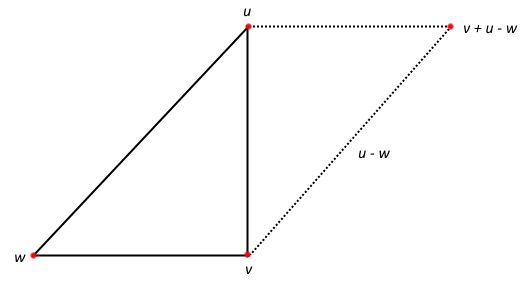
1. The Parallelogram Predictor
It turns out we can implement these predictors with only a small local amount of connectivity information and if we do them in the same pass as our index buffer encoding/decoding, this information is largely already there. If you recall the last post, most meshes had the vast majority of their triangles coming from an edge in the edge cache, so we can include the index to the third vertex of the triangle that edge came from in the FIFO and use that to perform parallelogram prediction.
This is fairly standard for mesh compression, as there is nearly always information used in the connectivity encoding that gives you a connected triangle. Some systems go a fair bit further, using full connectivity information and a multiple passes to produce more accurate vertex predictions.
For the rarer cases where there is not an edge FIFO hit, we can use another vertex in the triangle for delta prediction. It turns out only one vertex case (the first vertex in a new-new-new triangle) does not have a vertex relatively available to predict from. One of the advantages for this is that it keeps our compression working in the case where we don’t have many shared edges, albeit less efficiently.
One of the limitations of the parallelogram predictor is that the point it predicts is on the same plane as the triangle the prediction was based on. This means if your mesh has a large curve, there will be a reasonable amount of error. There are multiple ways to get around this problem; the original Touma and Gotsman paper used the 2 previously decoded edges closest to the direction of the edge adjacent the vertex to be decoded and averaged the “crease” direction of the triangles, then applied this to move the prediction. Other papers have used estimates from other vertices in the neighborhood and used more complex transform scheme. One paper transformed all the vertices to a basis space based on the predicting triangle, ran k-means to produce a limited set of prediction points, then encoded the index to the closest point along with the error. There are many options for improving the general prediction.
For my purposes though, I’m going to make an engineering decision to trade off a bit of compression for simplicity in the implementation and stick with the bare bones parallelogram predictor. There are a couple of reasons for this; firstly, it’s very easy to make the bare bones predictor with simple integer arithmetic (deterministic, fast and exact). You can apply it for each component, without referencing any of the others, and it works passing well for things like texture coordinates and some normal encodings.
One of the advantages about working with a vertex cache optimized ordering is that the majority of connected vertices have been recently processed, meaning they are likely in the cache when we reference them for decompression.
Entropy Encoding
Now, entropy encoding for the vertex data is quite a different proposition to what we used for connectivity data. Firstly, we aren’t using a set quantization pass, so straight up the probability distribution of our input is going to vary quite a lot. Secondly, as the distance between vertices in different meshes varies quite a lot, prediction errors are probably going to vary quite a lot. Thirdly, even with good predictors on vertex data you can have quite large errors for some vertices. All of this means that using a static probability distribution for error residuals is not going to fly.
Let’s look at the number of occurrences for residuals just for the parallelogram predictor, for the bunny model vertex positions, at 14 bits a component (graph below). We’ve applied a ZigZag encoding, such as used in protocol buffers, to allow us to encode negative residuals as positive numbers. The highest residual is 1712 (although there are many residuals below that value that don’t occur at all) and the number of unique residuals that occur is 547.
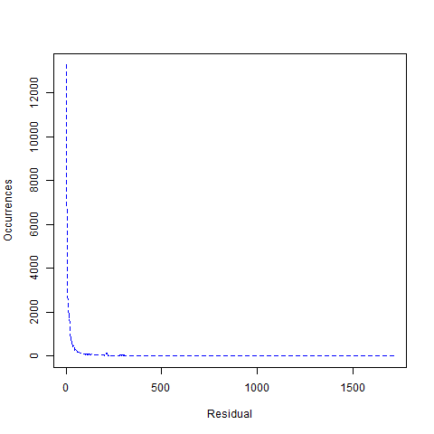
2. The Error Residuals for Vertex Positions of the Bunny Mesh
A fairly standard approach here would be to calculate the error residuals in one pass, while also calculating a histogram, which we could then use to build a probability distribution for a traditional entropy encoder, where we could encode the vertices in a second pass. This introduces another pass in encoding (we’ve already introduced one potentially for quantization), as well as the requirement to buffer residuals. It also means storing a code table (or probabilities/frequencies) in the compression stream. For our connectivity compressor we used Huffman and a table driven decoder, lets look at how that approach would work here.
If we feed the above data into a Huffman code generator, we end up with the longest code being 17bits, meaning we would need a table of 131072 entries (each of which would be larger than for our connectivity compression, because the residuals themselves are larger than a byte). That’s a bit steeper than our connectivity compression, but we could get the table size down using the approach outlined in Moffat and Turpin’s On the Implementation of Minimum Redundancy Prefix Codes paper, at the cost of an increase in complexity of the decoder. However, other models/quantization levels might require even larger tables.
But how would compression be? For just the position residuals for the parallelogram predicted vertices (which is 34634 of 34817 vertices) we would use 611,544 bits (not counting the code/frequency table, which would also be needed). That’s reasonable at 17.66 bits a vertex, or 5.89 bits a component (down from 14).
The compression is reasonable for this method (which we would expect, given it’s pedigree). But it brings with it some disadvantages; an extra encoding pass and buffering, storing a code table, extra complexity or a large decoding table as well as some overhead in decoding to build the decoding table.
Let’s take a different approach.
Universal codes allow any integer to be encoded, but each code ends up with an implied probability correlated to how many bits it uses. You can use them for fairly general entropy encoding where you know the rank of a set of codes, but they don’t perform as well as Huffman coding usually, because the probability distribution of real codes usually doesn’t match that of the universal codes exactly.
Exponential-Golomb codes are a kind of universal code with some interesting properties. They combine an Elias gamma code to represent the most significant bits of a value, with a fixed number of the lowest significant bits (k) encoded directly. Also, I dare you to try and type “Golomb” without inserting a “u”. The first part of the code is a unary code that will have quite a limited number of bits for our range of values, which we can use a bit scan instruction to decode instead of a table lookup, so we can build a fast decoder without running into memory problems (or cache miss problems).
Now, it turns out this is a good model for the case where you have a certain number of low bits which have approximately a uniform probability distribution (so they are quite noisy), with the bits above the k’th bit being increasingly unlikely to be switched on. The shortest length codes for a particular value are produced when the most significant bit also happens to be the top bit in a k-bits integer.
So, if we can correctly estimate what k should be for a particular component residual at a particular time, then we can get the best bit length encoding for that value. If we make the (not always correct) assumption that the traversal order of vertices means that similar vertices will be close together and that the residuals for each component are probably going to be similar in magnitude, then a moving average based off what the optimal k for the previous values were might be a reasonable way to estimate an optimal k (a kind of adaptive scheme, instead of a fixed code book).
I decided to go with an exponential moving average, because it requires very little state, no lookbacks and we can calculate certain exponential moving averages easily/quickly in fixed point (which we really want, for determinism, as we want to be able to reproduce the exact same k on decompression). After some experimentation and keeping in mind what we can calculate with shifts, I decided to go with an alpha of 0.125. In 16/16 fixed point, the moving average looks like this (where kEstimate is the k that would give the best encoding for the current value):
k = ( k * 7 + ( kEstimate << 16 ) ) >> 3;
Also, after a bit of experimentation, I went with a bit of a simplified version of exponential golomb coding that has a slightly better probability distribution (for our purposes) and is slightly faster to decode. Our code will have a unary code starting from the least significant bits, where the number of zeros will encode the number of bits above k that our residual will have. If that number is 0, what will follow will be k bits (representing the residual, padded out with zeros in the most significant bits to k bits). If it is more than zero, after will follow the residual without the most significant bit (which will be implied by the position we can calculate from the unary code).
Below are simplified versions of the encoding and decoding functions for this universal code. Note that we return the number of bits from writing the value, so we can feed it into the moving average as our estimate for k. The DecodeUniversal in this case uses the MSVC intrinsic for the bit scan, but in our actual implementation we also support the __builtin_ctz intrinsic from gcc/clang and a portable fallback (although, I need to test these platforms properly).
inline uint32_t WriteBitstream::WriteUniversal( uint32_t value, uint32_t k )
{
    uint32_t bits = Log2( ( value << 1 ) | 1 );

    if ( bits <= k )
    {
        Write( 1, 1 );
        Write( value, k );
    }
    else
    {
        uint32_t bitsMinusK = bits - k;

        Write( uint32_t( 1 ) << bitsMinusK, bitsMinusK + 1 );
        Write( value & ~( uint32_t( 1 ) << ( bits - 1 ) ), bits - 1 );
    }

    return bits;
}

inline uint32_t ReadBitstream::DecodeUniversal( uint32_t k )
{
    if (m_bitsLeft < 32)
    {
        uint64_t intermediateBitBuffer =
            *( reinterpret_cast< const uint32_t* >( m_cursor ) );

        m_bitBuffer |= intermediateBitBuffer << m_bitsLeft;

        m_bitsLeft  += 32;
        m_cursor    += 4;
    }

    unsigned long leadingBitCount;

    _BitScanForward( &leadingBitCount,
                     static_cast< unsigned long >( m_bitBuffer ) );

    uint32_t topBitPlus1Count = leadingBitCount + 1;

    m_bitBuffer >>= topBitPlus1Count;
    m_bitsLeft   -= topBitPlus1Count;

    uint32_t leadingBitCountNotZero = leadingBitCount != 0;
    uint32_t bitLength              = k + leadingBitCount;
    uint32_t bitsToRead             = bitLength - leadingBitCountNotZero;

    return Read( bitsToRead ) | ( leadingBitCountNotZero << bitsToRead );
}
There are a few more computations here than in a table driven Huffman decoder, but we get away without the table look-up memory access and the cache miss that could bring for larger tables. I am a fan of the adage “take me down to cache miss city where computation is cheap but performance is shitty”, so this sits a bit better with my performance intuitions for potentially unknown future usage.
But what sort of compression do we get? It turns out for this particular case, although definitely not all cases, our adaptive universal scheme actually outperforms Huffman, with a total of 604,367 bits (17.45 bits a vertex or 5.82 bits a component). You might ask how, given Huffman produces optimal codes (for whole bit codes) that we managed to beat it; the answer is that less optimal adaptive coding can beat better codes with a fixed probability distribution. In some cases it performs a few percent worse, but overall it’s competitive enough that I believe the trade offs for encoder/decoder simplicity and performance are worth it.
Encoding Normals
For encoding vertex normals I use the precise Octahedral encoding described in A Survey of Efficient Representations for Unit Vectors. This encoding works relatively well with parallelogram prediction, but has the problem of strange wrapping on the edges of the mapping, which makes prediction fail at the borders, meaning vertices on triangles that straddle those edges can end up with high residual values. However, the encoding itself is good enough it can stand up to a reasonable amount of quantization.
Because this encoding is done in the quantization pass (outside of the main encoder/decoder), it’s pretty easy to drop in other schemes of your own making.
Results
For now, I’m going to stick to just encoding positions and vertex normals (apart from the Armadillo mesh, which doesn’t have normals included), because the meshes we’ve been using for results up until this point don’t have texture coordinates. At some stage I’ll see about producing some figures for meshes with texture coordinates (and maybe some other vertex attributes).
First let’s look at the compression results for vertex positions at 10 to 16 bit per component. Results are given in average bits per component, to get the amount of storage for the final mesh, multiply the value by the number of vertices times 3. Note that the number for 14 bit components is slightly higher than that given earlier, because this includes all cases, not just those using parallelogram prediction.
| MODEL | VERTICES | 10 bit | 11 bit | 12 bit | 13 bit | 14 bit | 15 bit | 16 bit |
|---|---|---|---|---|---|---|---|---|
| Bunny | 34,817 | 2.698 | 3.280 | 4.049 | 4.911 | 5.842 | 6.829 | 7.828 |
| Armadillo | 172,974 | 2.231 | 2.927 | 3.765 | 4.553 | 5.466 | 6.290 | 7.209 |
| Dragon | 438,976 | 2.640 | 3.438 | 4.297 | 5.292 | 6.306 | 7.327 | 8.351 |
| Buddha | 549,409 | 2.386 | 3.123 | 4.037 | 5.014 | 6.017 | 7.032 | 8.055 |
Now lets look at normals for bunny, dragon and buddha, from 8 to 12 bits a component, using the precise octahedral representation (2 components). Note that the large predictions errors for straddling edges cause these to be quite a bit less efficient than positions, although normals do not predict as well with the parallelogram predictor in general.
| MODEL | VERTICES | 8 bit | 9 bit | 10 bit | 11 bit | 12 bit | |
|---|---|---|---|---|---|---|---|
| Bunny | 34,817 | 4.840 | 5.817 | 6.813 | 7.814 | 8.816 | |
| Dragon | 438,976 | 4.291 | 5.255 | 6.250 | 7.251 | 8.252 | |
| Buddha | 549,409 | 4.664 | 5.632 | 6.627 | 7.627 | 8.628 | |
Now, let’s look at decompression speeds. Here are the speeds for the Huffman table driven index buffer compression alone. Note, there has been one or two optimisations since last time that got the speed closer to the fixed width code version.
| MODEL | TRIANGLES | UNCOMPRESSED | COMPRESSED | COMPRESSION TIME | DECOMPRESSION TIME (MIN) | DECOMPRESSION TIME (AVG) | DECOMPRESSION TIME (MAX) | DECOMPRESSION TIME (STD-DEV) |
|---|---|---|---|---|---|---|---|---|
| Bunny | 69,630 | 835,560 | 70,422 | 2.71ms | 0.551ms | 0.578ms | 0.623ms | 0.030ms |
| Dragon | 871,306 | 10,455,672 | 875,771 | 31.7ms | 7.18ms | 7.22ms | 7.46ms | 0.060ms |
| Buddha | 1,087,474 | 13,049,688 | 1,095,804 | 38.9ms | 8.98ms | 9.02ms | 9.25ms | 0.058ms |
Here are the figures where we use quantization to reduce vertices down to 14 bits a component and normals encoded as described above in 10 bits a component, then run them through our compressor. Timings and compressed size include connectivity information, but timings don’t include the quantization pass. Uncompressed figures are for 32 bit floats for all components, with 3 component vector normals.
| MODEL | TRIANGLES | UNCOMPRESSED | COMPRESSED | COMPRESSION TIME | DECOMPRESSION TIME (MIN) | DECOMPRESSION TIME (AVG) | DECOMPRESSION TIME (MAX) | DECOMPRESSION TIME (STD-DEV) |
|---|---|---|---|---|---|---|---|---|
| Bunny | 69,630 | 1,671,168 | 206,014 | 5.20ms | 1.693ms | 1.697ms | 1.795ms | 0.015ms |
| Dragon | 871,306 | 20,991,096 | 2,598,507 | 62.87ms | 21.25ms | 21.29ms | 21.36ms | 0.015ms |
| Buddha | 1,087,474 | 26,235,504 | 3,247,973 | 79.75ms | 26.83ms | 27.00ms | 28.79ms | 0.44ms |
Also, here’s an interactive demonstration that shows the relative quality of a mesh that has been round-tripped through compression with 14 bit component positions/10 bit component normals as outlined above (warning, these meshes are downloaded uncompressed, so they are several megabytes).
At the moment, I think there is still some room for improvement, both compression wise and performance wise. However, I do think it’s close enough in both ballparks to spark some discussions of the viability. One of the things to note is that the compression functions still provide the vertex re-mapping, so it is possible to store vertex attributes outside of the compressed stream.
It should be noted, the connectivity compression doesn’t support degenerate triangles (a triangle with two or more of the same vertex indices), which is still a limitation. As these triangles don’t add anything visible to a mesh, it is usually alright to remove them, but there are some techniques that might take advantage of them.
A Quick Word on an Interesting Variant
I haven’t investigated this thoroughly, but there is an interesting variant of the compression that gets rid of the free vertex (vertex cache miss) cases and treats them the same as a new vertex case. This would mean encoding some vertices twice, but as the decoding is bit exact the end result would be the same. Because these vertex reads are less frequent than their new vertex cousins (less than a third than in the bunny), it means that the overhead would be relatively small and still a fair bit smaller than the uncompressed result (and you would gain something back on the improved connectivity compression). However, it would mean that you could decode vertices only looking at those referenced by the FIFOs (which would be whole triangles in the case of the edge FIFOs) and that essentially you could reduce processing/decompression to a small fixed size decompression state and always forward reading from the compressed stream.
The requirement for large amounts of state (of potentially unknown size), as well as large tables for Huffman decoding, is part of what has made hardware support for mesh decompression a non-starter in the past.
Wrapping Up
There are a lot of details that didn’t make it into this post, due to to time poverty, so if you are wondering about anything in particular, leave a comment or contact me on twitter and I will try to fill in the blanks. I was hoping to get more into the statistics behind some of the decisions made (including some interactive 3D graphs made with R/rgl that I have been itching to use), but unfortunately I ran out of time.
blog comments powered by Disqus