Cramming Entropy Encoding into Index Buffer Compression
I was never really happy with the compression ratio achieved in the Vertex Cached Optimised Index Buffer Compression algorithm, including the improved version, even though the speed was good (if you haven’t read these posts, this one might not make sense in places). One of the obvious strategies to improve the compression was to add some form of entropy encoding. The challenge was to get a decent boost in compression ratio while keeping decoding and encoding speed/memory usage reasonable.
Index buffers may not seem at first glance to be that big of a deal in terms of size, but actually they can be quite a large proportion of a mesh, especially for 32bit indices. This is because on average there are approximately 2 triangles for each vertex in a triangle mesh and each triangle takes up 12 bytes.
Note, for the remainder of this post I’ll be basing the work on the second triangle code based algorithm, that currently does not handle degenerate triangles (triangles where 2 vertices are the same). It is not impossible to modify this algorithm to support degenerates, but that will be for when I have some more spare time.
Probability Distributions
From previous work, I had a hunch about what the probability distribution for the triangle codes was, with the edge/new vertex code being the most likely and the edge/cache code being almost as frequent. During testing, collected statistics showed this was indeed the case. In fact, for the vertex cache optimised meshes tested, over 98% of the triangle codes were one of the edge codes (including edge/free vertex, but in a much lower proportion).
Entropy encoding on the triangle codes alone wouldn’t be enough to make much of a difference (given the triangle code is only 4 bits and the average triangle about 12.5 in the current algorithm), without reducing the amount of space used by the edge and vertex cache FIFO index entries. Luckily, Tom Forsyth’s vertex cache optimisation algorithm (explained here) is designed to take advantage of multiple potential cache sizes (32 entries or smaller), meaning it biases towards more recent cache entries (as that will cause a hit in both the smaller and larger caches).
The probability distributions (charted below, averaged over a variety of vertex cache optimised meshes) are quite interesting. Both show a relatively geometric distribution with some interesting properties: Vertex FIFO index 0 is a special case, largely due to it being the most common vertex in edge cache hits. Also, the 2 edges usually going into the edge cache for a triangle (the other edge is usually from the cache already) share very similar probabilities, making the distribution step down after every second entry. Overall these distributions are good news for entropy encoding, because all of our most common cases are considerably more frequent than our less common ones.
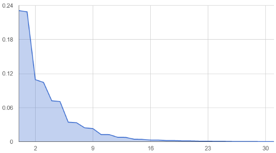
1. Edge FIFO Index Probability Distribution
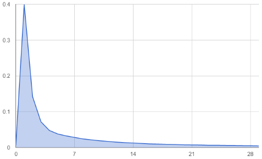
2. Vertex FIFO Index Probability Distribution
The probability distributions were similar enough between meshes optimised with Tom’s algorithm that I decided to stick with a static set of probability distributions for all meshes. This has some distinct advantages; there is no code table overhead in the compression stream (important for small meshes) and we can encode the stream in a single pass (we don’t have to build a probability distribution before encoding).
One of the other things that I decided to do was drop the Edge 0/New Vertex and Edge 1/New Vertex codes, because it was fairly clear from the probability distributions that these codes would actually end up decreasing the compression ratio later on.
Choosing a Coding Method
Given all of this, it was time to decide on an entropy encoding method. There are a few criterion I had in picking an entropy encoding scheme:
- The performance impact on decoding needed to be small.
- The performance impact on encoding reasonable enough that on-the-fly encoding was still plausible.
- Low fixed overheads, so that small meshes were not relatively expensive.
- Keep the ability to stream out individual triangles (this isn’t implemented, but is not a stretch).
- Low state overhead (for the above).
- Switching alphabets/probability distributions multiple times for a single triangle (required because we have multiple different codes per triangle).
- Single pass for both encoding and decoding (i.e. no having to buffer up intermediates).
Traditionally the tool for a job like this would be a prefix coder, using Huffman codes. After considering the alternatives, this still looked like the best compromise, with ANS requiring the reverse traversal (meaning two passes for encoding) and other arithmetic and range encoding variants being too processor intensive/a pain to mix alphabets. Another coding considered was a word aligned coding that used the top bits of a word (32 or 64 bits) to specify the bit width of codes put into the rest of the word. This coding is simple, but would require some extra buffering on encoding.
After generating the codes for the probability distributions above, I found the maximum code-lengths for the triangle codes were 11 bits. One of the things about the triangle codes was that there were a fair few codes that were rare enough that they were essentially noise, so I decided to smooth the probability distribution down a bit at the tail (a kind of manual length limiting, although it’s perfectly possible to generate length limited Huffman codes), which reduced the maximum code lengths to 7 bits, with the 3 most common cases taking up 1, 2 or 3 bits respectively (edge/new, edge/cached, edge/free).
The edge FIFO indices came in at a maximum code length of 11 bits (with the most common 9 codes coming in between 2 and 5 bits) and the vertex FIFO indices came in with a maximum length of 8 bits (with the 7 most common codes coming in between 1 and 5 bits).
Implementing the Encoder/Decoder
Because the probability distributions are static, for the encoder we can just embed static/constant tables, mapping symbols to codes and code-lengths. These could then be output using the same bitstream code used by the old algorithm.
For the decoder, I decided to go with a purely table driven approach as well (it’s possible to implement hybrid decoders that are partially table driven, with fall-backs, but that would’ve complicated the code more than I would’ve liked). This method uses a table able to fit the largest code as an index and enumerates all the variants for each prefix code. This was an option because the maximum code lengths for the various alphabets were quite small, meaning that the largest table would have 2048 entries (and the smallest, 128). These tables are embedded in the code and are immutable.
To cut down on table space as much as possible (to be a good cache using citizen), each table entry contained two 1 byte values (the original symbol and the length of the code). In total, this means 2432 decoding table entries (under 5K memory use).
struct PrefixCodeTableEntry
{
    uint8_t original;
    uint8_t codeLength;
};
Symbols were encoded with the first bit in the prefix starting in the least significant bit. This made the actual table decoding code very simple and neat. The decoding code was integrated directly with the reading of the bit-stream, which made mixing tables for decoding different alphabets (as well as the var-int encodings for free-vertices) far easier than if each decoder was maintaining.
Here is a simplified version of the decoding code:
inline uint32_t ReadBitstream::Decode( const PrefixCodeTableEntry* table, uint32_t maxCodeSize )
{
    if ( m_bitsLeft < maxCodeSize )
    {
        uint64_t intermediateBitBuffer = *(const uint32_t*)m_cursor;

        m_bitBuffer |= intermediateBitBuffer << m_bitsLeft;
        m_bitsLeft  += 32;
        m_cursor    += sizeof(uint32_t);
    }

    uint64_t                    mask       = ( uint64_t( 1 ) << maxCodeSize ) - 1;
    const PrefixCodeTableEntry& codeEntry  = table[ m_bitBuffer & mask ];
    uint32_t                    codeLength = codeEntry.codeLength;

    m_bitBuffer >>= codeLength;
    m_bitsLeft   -= codeLength;

    return codeEntry.original;
}
Because m_bitBuffer is 64bits wide and the highest maxCodeSize in our case is 11 bits, we can always add in another 32bits at a time into the buffer without overflowing when we have less than the maximum code size left. This guarantees that we will always have at least the maximum code length of bits in the buffer, before we try and read from the table. I’ve used a 32 bit read from the underlying data here (which brings up endian issues etc), but the actual implementation only does this as a special case for x86/x64 currently (manually constructing the intermediate byte by byte otherwise).
Because we are always shifting codeLength bits out of the buffer afterwards, the least significant bits of the bit buffer will always contain the next code when we do the table read. The mask is to make sure we only use the maximum code length of bits to index the decoding table. With inlining (which we get a bit heavy handed with forcing in the implementation), the calculation of the mask should collapse down to a constant.
Results
Since last time there has been some bug fixes and some performance improvements for the triangle code algorithm (and I’ve started compiling in x64, which I should’ve been doing all along), so I’ll present the improved version as a baseline (all results are on my i7 4790K on Windows, compiled with Visual Studio 2013). Here we use 32 runs to get a value:
| MODEL | TRIANGLES | UNCOMPRESSED | COMPRESSED | COMPRESSION TIME | DECOMPRESSION TIME (MIN) | DECOMPRESSION TIME (AVG) | DECOMPRESSION TIME (MAX) | DECOMPRESSION TIME (STD-DEV) |
|---|---|---|---|---|---|---|---|---|
| Bunny | 69,630 | 835,560 | 108,908 | 2.42ms | 0.552ms | 0.558ms | 0.599ms | 0.0086ms |
| Armadillo | 345,944 | 4,151,328 | 547,781 | 12.2ms | 2.81ms | 2.82ms | 2.86ms | 0.0103ms |
| Dragon | 871,306 | 10,455,672 | 1,363,265 | 35.2ms | 7.22ms | 7.27ms | 7.51ms | 0.0724ms |
| Buddha | 1,087,474 | 13,049,688 | 1,703,928 | 38.8ms | 9.01ms | 9.04ms | 9.176ms | 0.0304ms |
So, our baseline is a fair bit faster than before. Throughput is currently sitting over 122 million triangles a second (on a single core), which for 32bit indices represents a decoding speed of ~1,400MiB/s and about 12.5 bits a triangle. Here’s the new entropy encoding variant:
| MODEL | TRIANGLES | UNCOMPRESSED | COMPRESSED | COMPRESSION TIME | DECOMPRESSION TIME (MIN) | DECOMPRESSION TIME (AVG) | DECOMPRESSION TIME (MAX) | DECOMPRESSION TIME (STD-DEV) |
|---|---|---|---|---|---|---|---|---|
| Bunny | 69,630 | 835,560 | 70,422 | 2.52ms | 0.827ms | 0.828ms | 0.844ms | 0.0029ms |
| Armadillo | 345,944 | 4,151,328 | 354,843 | 12.1ms | 4.15ms | 4.17ms | 4.27ms | 0.0303ms |
| Dragon | 871,306 | 10,455,672 | 875,771 | 31.8ms | 10.6ms | 10.64ms | 10.82ms | 0.0497ms |
| Buddha | 1,087,474 | 13,049,688 | 1,095,804 | 38.7ms | 13.25ms | 13.28ms | 13.788ms | 0.0687ms |
The new algorithm has throughput of a bit over 82 million triangles a second (so about 67% the throughput, ~940MiB/s), but gets very close to 8bits a triangle (so about 64% the size). There is virtually no overhead in the encoding time (with it even being slightly faster at times), probably due to less bits going into the bitstream. Considering our most common case in the old algorithm (edge/new vertex) was 9 bits, this is a considerable gain compression wise.
Conclusion
Overall, this algorithm is still not near the best indice compression algorithms in terms of compression ratio (which get less than a bit a triangle, when using adaptive arithmetic encoding), however it is fast, relatively simple (I don’t think an implementation in hardware would be impossible), requires very little in the way of state overhead/supporting data-structures/connectivity information and allows arbitrary topologies/triangle orderings (other algorithms often change the order of the triangles). Although, it is obviously focused on vertex cache optimised meshes, which happens to be the triangle ordering people want meshes in. The next step is probably to add vertex compression and create a full mesh compression algorithm, as well as handling degenerates with this algorithm.
As usual, the code for this implementation can be seen on GitHub.
blog comments powered by Disqus